
Measuring point overlap
Patterns of overlap among occurrence points
For different lines of research that I’ve been involved with lately (morphological differences between co-occurring species of yellow-shouldered bat and the spatial patterning between virus records in wild mammals and human viral cases), I’ve been thinking about spatial overlap between point occurrence data and how to quantify it.
Fortunately, in this recent and very cool paper Marcel Cardillo and Dan Warren introduced a nifty method to quantify overlap among species using the proximity of occurrence points using patterns of co-aggregation for multiple species: The point-proximity metric O.
In my opinion, using point occurrences to represent species’ distributions is usually the way to go because: (1) sometimes point occurrences is all we have, and (2) polygon range maps might overestimate distributions and lead to various errors in downstream analyses. If anyone is interested, I summarized the pros and cons of point data in this 2015 paper on lagomorphs.
Another very nice feature of the O metric is that it works on 2d space in general, so we can use it to measure overlap in environmental or even morphological space (usually defined by principal components i.e. points on two axes).
In the appendix of the Cardillo and Warren paper, they break down the behaviour of the O statistic and its sensitivity to different levels of clumping and to the asymmetry in the distribution of points among the two species. I wanted to use the O statistic with my data, but despite the clear explanation in the text and the simulations in the appendix, I was still slow to grasp how the range of values corresponds with different levels of overlap. As stated in the paper:
“The value of O is bounded between zero and one, with values close to zero indicating little spatial overlap while a value of ~0.5 is expected if the occurrence points of the two species are randomly and independently distributed across the same area.”
I believe that O will get a lot of use in the future and I hope this post helps others looking to use it (I also hope I didn’t mess anything up). All the code needed to recreate the two figures in this post is in the embedded gist at the end, as long as you have the required packages it should be fully reproducible.
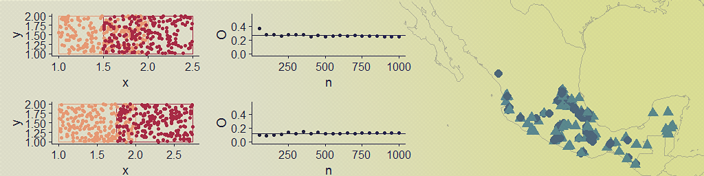
To visualize and test O for different degrees of polygon overlap and a varying number of points, I generated random points within two polygons of equal areas with varying degrees of overlap (accomplished by simply shifting one of the polygons along the x axis).
With this hastily-put together function and plotting code, I was able to visualize the occurrence points alongside a plot of how O behaves with different numbers of points. In this case there is no asymmetry in the sample sizes for each ‘species’.
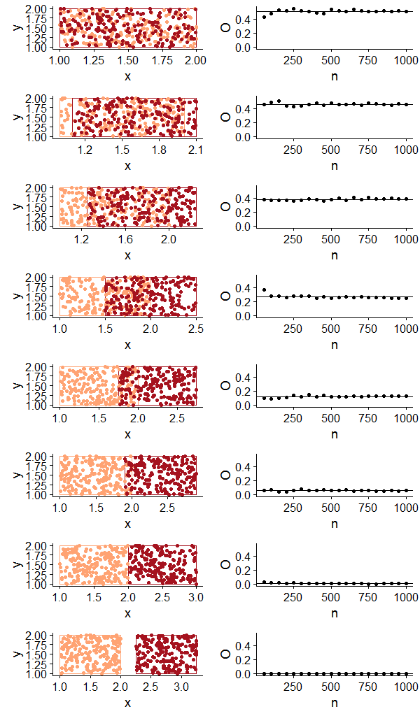
The resulting plot is pretty much what I expected to see, but I still found it helpful to see how O increases with increasing spatial overlap and how we get similar values even for small(ish) sample sizes. Now for a somewhat silly example with real distributions, I used rgbif to download point occurrence data for a few species with varying degrees of overlap. I chose two species of bird and three species of mammal that would show the range of values of O with real data.
The two bird species have a narrow contact zone, and each of these has a slight amount of point overlap with the mouse opossum. These three in turn have no overlap at all with the remaining two arid zone rodents, which show a fair amount of overlap.
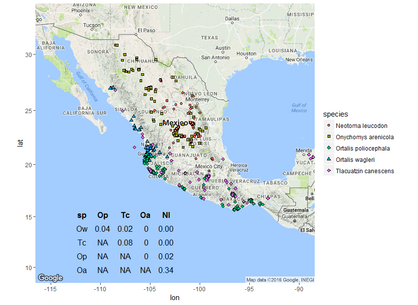
I was unfamiliar with the inset function for plotting custom objects inside a ggmap, but it turned out to be pretty useful and I’ll be using it in the future.
Another relevant method for examining the co-distribution of point occurrences involves Ripley’s K and L functions, descriptive statistics for detecting deviations from spatial homogeneity. These are also based on Euclidean distances, and they can be used in cases in which sampling is biased. I’ll write a post about these methods in the future, but anyone interested should check out these two links.
All the code is below, contact me with any questions, comments, or if the code isn’t working.
#Code and data