
This recent post by Jeremy Selva shows a nice workflow for working with problematic formatted spreadsheets in R.
I’ve worked on this topic before, so I when I saw the post I had to meddle. I suggested using functions from the unheadr package to address some of these issues. They didn’t work because of assumptions I hard-coded into the package, but these are fixed now. These fixes are part of unheadr v0.4.0. To demonstrate the functions and also to celebrate 20k downloads (🥳), here is my take (with the benefit of hindsight) on tackling this troublesome spreadsheet. ALL CREDIT TO JEREMY FOR COMING UP WITH THE EXAMPLE AND WORKFLOW.
The spreadsheet/workbook in question can be downloaded from Jeremy’s GitHub here.
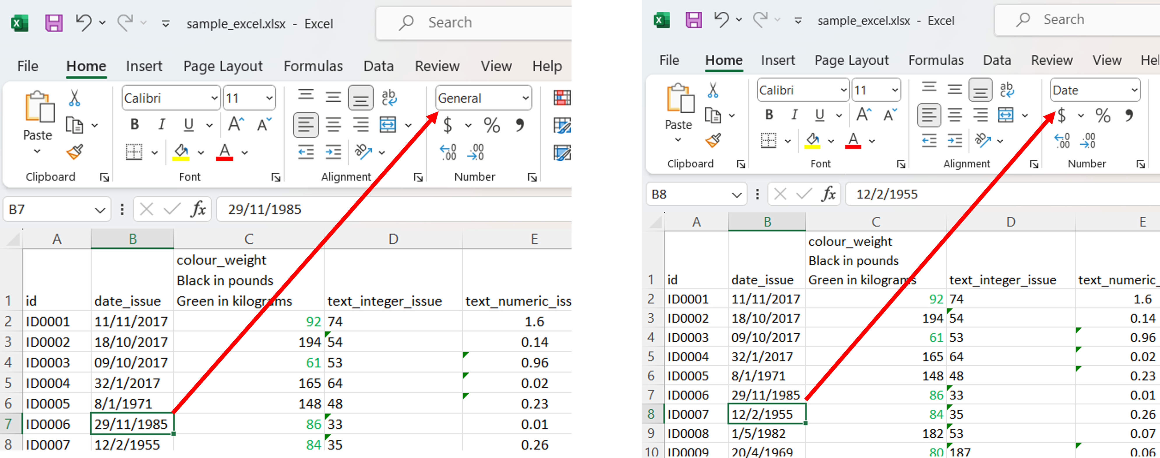
For context, I’m reproducing the images from the original post about the issues with the data, which are good examples of:
😢 Things we shouldn’t do but which happen anyway in spreadsheets:
1. A date variable with different cell formats, plus whatever strange thing Excel does to dates.
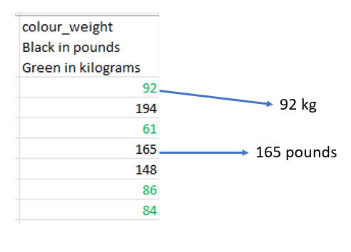
2. Meaningful formatting
Using text color (and nothing else) to indicate units.
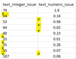
3. Numeric variables with some cells formatted as text.
These issues vary in how hard they are to address in downstream analyses, but as they accumulate we are more tempted to give up and work with the file directly in Excel (or Calc).
Here’s my take, which can be a complement to the stricter approach in Jeremy’s post.
First, read the spreasheet with readxl. Out of caution, we can read everything as text initially.
# load some useful packages
library(readxl)    # CRAN v1.4.3
library(lubridate) # CRAN v1.9.3
library(janitor)   # CRAN v2.2.0
library(readr)     # CRAN v2.1.5
library(dplyr)     # CRAN v1.1.4
library(tidyxl)    # CRAN v1.0.10
library(stringr)   # CRAN v1.5.1
library(tidyr)     # CRAN v1.3.1
library(unheadr)   # CRAN v0.4.0

samp <- read_excel("sample_excel.xlsx", col_types = "text")
Next, type_convert() from readr does a good job of parsing variables in a data frame, and has good heuristics to interpret numeric variables even when these had problematic combinations of cell formatting in the spreadsheet.
samp <- readr::type_convert(samp)── Column specification ────────────────────────────────────────────────────────────
cols(
id = col_character(),
date_issue = col_character(),
`colour_weight
Black in pounds
Green in kilograms` = col_double(),
text_integer_issue = col_double(),
text_numeric_issue = col_double(),
numeric_integer_issue = col_double(),
one_or_zero_issue = col_double()
)To fix the awkward date, lubridate can handle the dates that were imported more or less properly, and the excel_numeric_to_date() function from janitor was purpose-built to transform the dates stored as weird numbers. Afterwards we put the two together.
samp$newdate <- lubridate::parse_date_time(samp$date_issue,
  orders = c("ymd", "dmy")
)
samp$xldate <- excel_numeric_to_date(as.numeric(as.character(samp$date_issue)),
  date_system = "modern"
)
samp <- samp %>%
  mutate(date_fixed = coalesce(newdate, xldate)) %>%
  select(-newdate, -xldate, -date_issue)
> samp %>% select(date_fixed)
# A tibble: 1,053 × 1
date_fixed
<dttm>
1 2017-11-11 00:00:00
2 2017-10-18 00:00:00
3 2017-10-09 00:00:00
4 NA
5 1971-01-08 00:00:00
6 1985-11-29 00:00:00
7 1955-02-12 00:00:00
8 1982-05-01 00:00:00
9 1969-04-20 00:00:00
10 1962-11-21 00:00:00
# ℹ 1,043 more rows
# ℹ Use `print(n = ...)` to see more rowsLastly, there’s the issue of units of measurment for a variable encoded as text formatting. In this case the text color indicates the units. This information is lost when reading only the cell values with readxl, but we can embed the color code from each cell as a text annotation using the annotate_mf functions from unheadr.
> annotate_mf_all("sample_excel.xlsx")
Error in annotate_mf_all("sample_excel.xlsx") :
  Check spreadsheet for blank cells in seemingly empty rows
If we run annotate_mf_all() with the path to the spreadsheet, we’ll get an error message. Apparently there are formatted cells outside of the data rectangle, which is what readxl focuses on during the data import.
We can use tidyxl to unravel the problem, looking at the tail end of the output, we see some blank-formatted cells in rows 1054 and 1055, even though our samp data frame only has 1053 rows. These formatted cells create “ghost” rows that trip up the functions from unheadr.
> nrow(samp)
[1] 1053
spsheetcells <- tidyxl::xlsx_cells("sample_excel.xlsx")
spsheetcells %>%
select(row, is_blank, data_type) %>%
tail(10)# A tibble: 10 × 3
row is_blank data_type
<int> <lgl> <chr>
1 1053 FALSE numeric
2 1054 FALSE character
3 1054 FALSE character
4 1054 FALSE numeric
5 1054 FALSE numeric
6 1054 FALSE numeric
7 1054 FALSE numeric
8 1054 FALSE numeric
9 1055 TRUE blank
10 1056 TRUE blank After opening the file directly in a spreadsheet program and deleting the problem rows altogether (I saved this as a new file called sample_excel_cln.xlsx), the annotate_mf_all() function is able to translate the colorful text into a text annotation of the hex8 code for each color.
samp_format <- annotate_mf_all("sample_excel_cln.xlsx")Let’s have a look
samp_format[, 3]> samp_format[, 3]
# A tibble: 1,053 × 1
`colour_weight \nBlack in pounds\nGreen in kilograms`
<chr>
1 (color-FF00B050) 92
2 (color-FF000000) 194
3 (color-FF00B050) 61
4 (color-FF000000) 165
5 (color-FF000000) 148
6 (color-FF00B050) 86
7 (color-FF00B050) 84
8 (color-FF000000) 182
9 (color-FF00B050) 80
10 (color-FF00B050) 78
# ℹ 1,043 more rows
# ℹ Use `print(n = ...)` to see more rowsIf we drop the FF from the color codes (it’s shorthand for 100% opacity), recent versions of R Studio will preview a color right in the editor, so now we know which values are green and which are black.
“FF00B050” is green and “FF000000” is black
Let’s separate color code and weight value into their own columns:
samp_format <- samp_format %>%
  separate(`colour_weight
Black in pounds
Green in kilograms`, into = c("hex8code", "weight"), sep = " ") %>%
  mutate(weight = parse_number(weight))
> samp_format %>% select(id, hex8code, weight)
# A tibble: 1,053 × 3
id hex8code weight
<chr> <chr> <dbl>
1 (color-FF000000) ID0001 (color-FF00B050) 92
2 (color-FF000000) ID0002 (color-FF000000) 194
3 (color-FF000000) ID0003 (color-FF00B050) 61
4 (color-FF000000) ID0004 (color-FF000000) 165
5 (color-FF000000) ID0005 (color-FF000000) 148
6 (color-FF000000) ID0006 (color-FF00B050) 86
7 (color-FF000000) ID0007 (color-FF00B050) 84
8 (color-FF000000) ID0008 (color-FF000000) 182
9 (color-FF000000) ID0009 (color-FF00B050) 80
10 (color-FF000000) ID0010 (color-FF00B050) 78
# ℹ 1,043 more rows
# ℹ Use `print(n = ...)` to see more rowsNow we can conditionally convert pounds to kilograms, then remove the color annotation from the id variable, which we’ll use to merge this object with the dataframe we were working on initially.
samp_format <-
  samp_format %>%
  mutate(weight = round(if_else(str_detect(hex8code, "00B050"),
    weight, weight * 0.453
  ), 0)) %>%
  mutate(id = str_remove_all(id, "^[^\\s]+ ")) %>% # regex!
  select(id, weight)
> samp_format
# A tibble: 1,053 × 2
id weight
<chr> <dbl>
1 ID0001 92
2 ID0002 88
3 ID0003 61
4 ID0004 75
5 ID0005 67
6 ID0006 86
7 ID0007 84
8 ID0008 82
9 ID0009 80
10 ID0010 78
# ℹ 1,043 more rows
# ℹ Use `print(n = ...)` to see more rowsAfter joining the two objects, some minor cleanup of the names leaves us with nice and usable data.
sampjnd <- left_join(samp, samp_format) %>% clean_names()
sampjnd <-
  sampjnd %>% select(id,
    date = date_fixed, weight_kg = weight, text_integer_issue, text_numeric_issue, numeric_integer_issue,
    one_or_zero_issue
  )
names(sampjnd) <- str_remove(names(sampjnd), "_issue$")
> sampjnd
# A tibble: 1,053 × 7
id date weight_kg text_integer text_numeric numeric_integer
<chr> <dttm> <dbl> <dbl> <dbl> <dbl>
1 ID0001 2017-11-11 00:00:00 92 74 1.6 1
2 ID0002 2017-10-18 00:00:00 88 54 0.14 55
3 ID0003 2017-10-09 00:00:00 61 53 0.96 9
4 ID0004 NA 75 64 0.02 2
5 ID0005 1971-01-08 00:00:00 67 48 0.23 3
6 ID0006 1985-11-29 00:00:00 86 33 0.01 7
7 ID0007 1955-02-12 00:00:00 84 35 0.26 1
8 ID0008 1982-05-01 00:00:00 82 53 0.07 3
9 ID0009 1969-04-20 00:00:00 80 187 0.06 75
10 ID0010 1962-11-21 00:00:00 78 141 0.01 23
# ℹ 1,043 more rows
# ℹ 1 more variable: one_or_zero <dbl>
# ℹ Use `print(n = ...)` to see more rowsIf it’s not too late, following good practices for Data organization in spreadsheets will avoid a lot of pain. Otherwise, tools like the ones shown here can be useful.
All feedback welcome and again thanks to Jeremy Selva for the idea and GitHub issue that sparked all of this.
Further reading:
- Jenny Bryan’s Spreadhseet Resources
- Please don’t do this: Three common bad practices in sharing tables and spreadsheets and how to avoid them