
Update - January 2020: The
raster_functions fromnngeowere moved togeobgu. Thanks to @imaginary_nums for pointing this out.
This is an update to a previous Spanish-language post for working with spatial raster and vector data in R, prompted by recent developments such as the stars package, its integration with sf and raster, and a particularly useful wrapper in geobgu.
Extracting the underlying values from a raster is a fairly common task, so here is a workflow to calculate and extract values (mean, max, min, etc.) from a raster file across the distribution of a few different primate species in Mexico and Central America (“Mesoamerica”), loaded from a .shp file into a simple feature collection.
We use a single raster file with gridded values for the Human Footprint index (a compound measure of direct and indirect human pressures on the environment globally), calculated for 2009 by Venter et al. (2016), and a multipolygon shapefile of mammalian distribution maps downloaded from the IUCN Red List Spatial Data and Mapping Resources page (free & open download for educational use but an account is needed). All the required packages can be installed from CRAN, so this example can be reproduced by everyone (willing to download these large amounts of data).
These are the main steps in the process:
Load raster and polygon data
First, read_stars() can read the geotiff raster file into a stars object and st_read() to load the shapefile. Country boundaries can be loaded from rnaturalearth. All the polygons were projected into Mollweide +proj to match the raster.
# load packages
library(sf) # Simple Features for R
library(rnaturalearth) # World Map Data from Natural Earth
library(here) # A Simpler Way to Find Your Files
library(stars) # Spatiotemporal Arrays, Raster and Vector Data Cubes
library(dplyr) # A Grammar of Data Manipulation
library(ggplot2) # Create Elegant Data Visualisations Using the Grammar of Graphics
library(ggnewscale) # Multiple Fill and Color Scales in 'ggplot2'
library(scico) # Colour Palettes Based on the Scientific Colour-Maps
library(geobgu) # install from GitHub ("michaeldorman/geobgu")
library(ggrepel) # Automatically Position Non-Overlapping Text Labels with 'ggplot2'

# load raster
humanFp <- read_stars("path-to-the-data/HFP2009.tif")

# world map
worldmap <- ne_countries(scale = "small", returnclass = "sf")
mesoam <- worldmap %>%
  filter(region_wb == "Latin America & Caribbean" &
    subregion != "South America" &
    subregion != "Caribbean") %>%
  select(admin) %>%
  st_transform("+proj=moll")

# species ranges
mammalpolys <- st_read("path-to-the-data/TERRESTRIAL_MAMMALS.shp")
primate_polys <- filter(mammalpolys, order_ == "PRIMATES") %>% st_transform("+proj=moll")
Mask and crop the raster layer
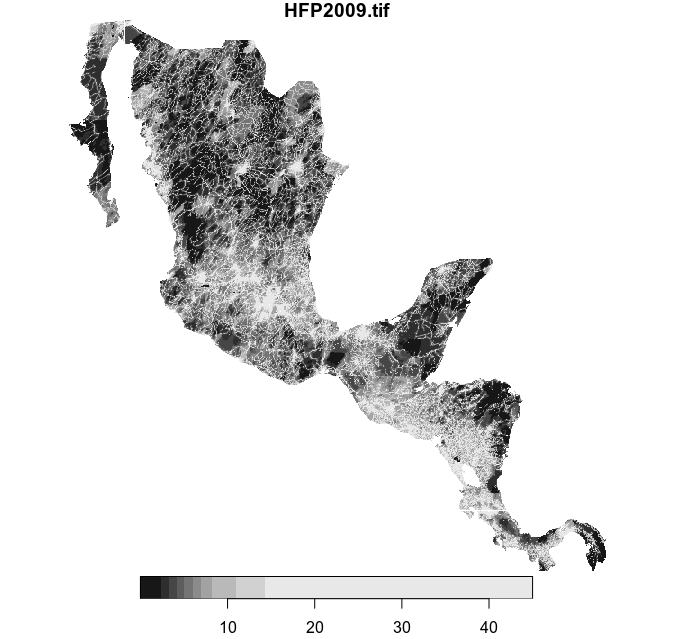
We only need raster data for our study region, so we can crop it using st_crop().
# crop the raster
hfp_meso <- st_crop(humanFp, mesoam)
plot(hfp_meso)
This is the cropped raster:
Subset the multipolygon feature collection
Immediately after loading the mammal range maps we used a simple dplyr operation to keep only the primates (our Order of interest), now we can spatially subset the data to keep only the polygons within our study area. Afterwards we group by species and summarize their geometries (this operation goes by many names in traditional GIS jargon, such as dissolve or aggregate).
# Mesoamerican species
primates_meso <- st_intersection(primate_polys, mesoam)
primates_meso <- primates_meso %>%
group_by(binomial) %>%
summarize()
# country outlines
divpol <-
worldmap %>%
filter(region_un == "Americas") %>%
select(admin) %>%
st_transform("+proj=moll")
# plotting limits
limsMeso <- st_bbox(st_buffer(primates_meso, 20000))
# species labels
labelling <- primates_meso %>% st_centroid()
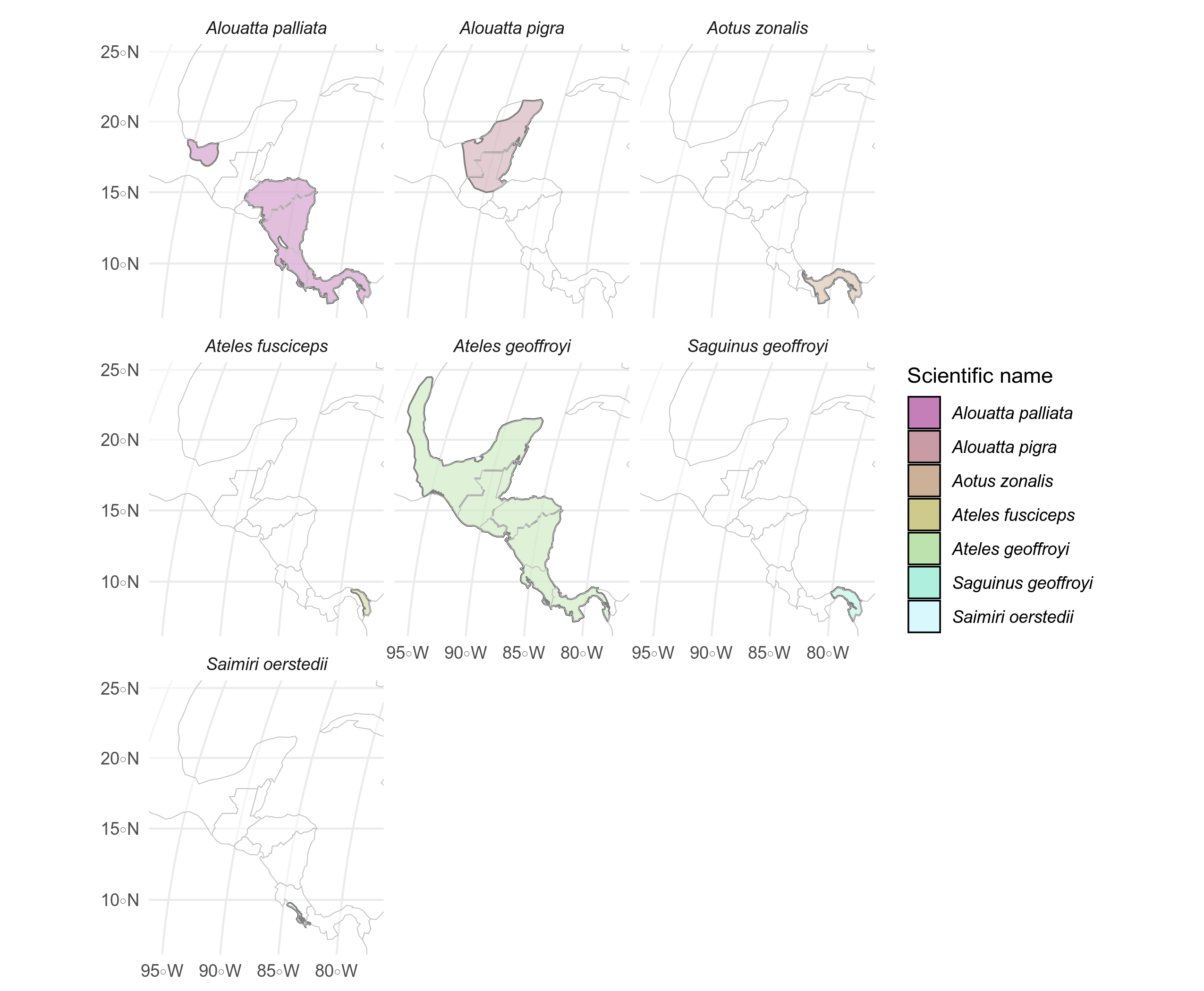
labelling <- labelling %>% mutate(X = st_coordinates(labelling)[, 1], Y = st_coordinates(labelling)[, 2])Because they overlap, we can make a faceted plot of the seven species present in the study area to see their ranges.
  ggplot() +
  geom_sf(data = primates_meso, aes(fill = binomial), alpha = 0.5, color = "black", size = 0.4) +
  facet_wrap(~binomial) +
  geom_sf(data = divpol, color = "gray", fill = "transparent", size = 0.2, alpha = 0.5) +
  coord_sf(
    xlim = c(limsMeso["xmin"], limsMeso["xmax"]),
    ylim = c(limsMeso["ymin"], limsMeso["ymax"])
  ) +
  scale_fill_scico_d(name = "Scientific name", palette = "hawaii") +
  theme_minimal() + theme(
    strip.text = element_text(face = "italic"),
    legend.text = element_text(face = "italic")
  )
Extract the underlying raster values for each feature in the polygon layer
The raster_extract() function comes in handy to apply raster::extract() on stars objects. It’s used here inside mutate to add new variables with the extracted values for each species (it’s vectorized for each feature 😎).
primates_meso <-
  primates_meso %>% mutate(
    hfpMean = raster_extract(hfp_meso, primates_meso, fun = mean, na.rm = TRUE),
    hfpMax = raster_extract(hfp_meso, primates_meso, fun = max, na.rm = TRUE),
    hfpMin = raster_extract(hfp_meso, primates_meso, fun = min, na.rm = TRUE)
  )
 primates_meso %>%
  st_set_geometry(NULL) %>%
  knitr::kable()
We can pull the data sans the geometry using st_set_geometry(NULL) and have a look at the extracted values.
| binomial | hfpMean | hfpMax | hfpMin |
|---|---|---|---|
| Alouatta palliata | 9.087961 | 50.00000 | 0.000000 |
| Alouatta pigra | 5.716039 | 47.00000 | 0.000000 |
| Aotus zonalis | 7.390708 | 42.41053 | 1.000000 |
| Ateles fusciceps | 3.870575 | 18.04213 | 1.000000 |
| Ateles geoffroyi | 8.495973 | 50.00000 | 0.000000 |
| Saguinus geoffroyi | 6.306356 | 42.41053 | 1.000000 |
| Saimiri oerstedii | 10.727800 | 40.78853 | 3.002395 |
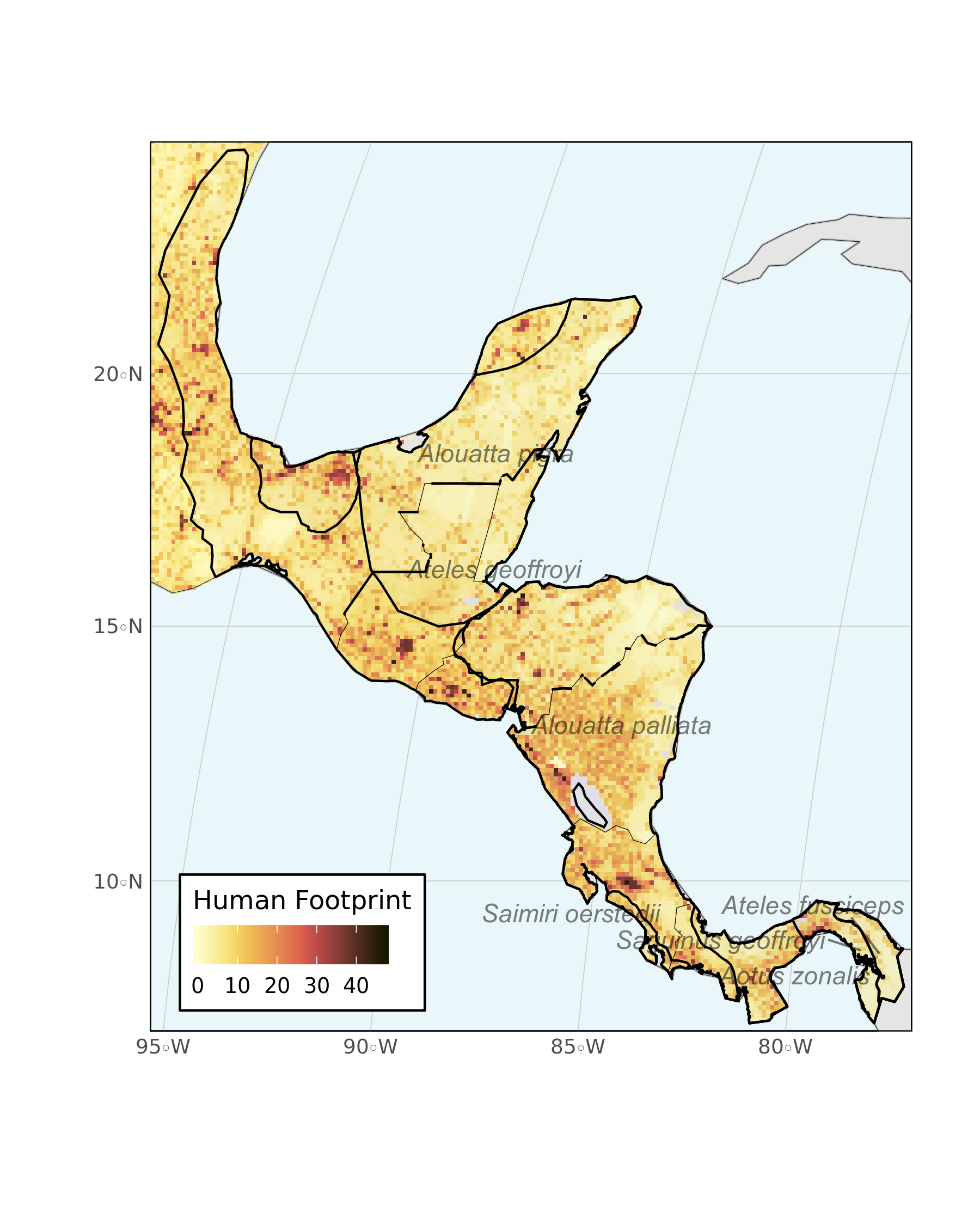
Lastly, we can plot everything together with ggplot2. This quick and simple map could be customized further with various grammar of graphics touches, but for now it looks pretty good.
  ggplot() +
  geom_sf(data = divpol, color = "gray", fill = "light grey") +
  geom_stars(data = hfp_meso, downsample = 10) +
  scale_fill_scico(
    palette = "lajolla", na.value = "transparent",
    name = "Human Footprint",
    guide = guide_colorbar(
      direction = "horizontal",
      title.position = "top"
    )
  ) +
  guides(fill = guide_colorbar(title.position = "top")) +
  new_scale_fill() +
  geom_sf(data = primates_meso, aes(group = binomial), color = "black", fill = "blue", alpha = 0.01) +
  geom_sf(data = divpol, color = "black", fill = "transparent", size = 0.1) +
  geom_text_repel(data = labelling, aes(X, Y, label = binomial), alpha = 0.5, fontface = "italic") +
  hrbrthemes::theme_ipsum_ps() + labs(x = "", y = "") +
  coord_sf(
    xlim = c(limsMeso["xmin"], limsMeso["xmax"]),
    ylim = c(limsMeso["ymin"], limsMeso["ymax"])
  ) +
  scale_x_discrete(expand = c(0, 0)) +
  scale_y_discrete(expand = c(0, 0)) +
  theme(
    legend.position = c(0.2, 0.1),
    panel.background = element_rect(fill = "#EAF7FA"),
    panel.border = element_rect(colour = "black", fill = "transparent"),
    legend.background = element_rect(fill = "white")
  )
One last plot, again using one facet per species to avoid overlap. Note the use of ggnewscale functions to use one fill for the raster and one for the polygon features.
ggplot()+
  geom_sf(data=divpol,color="gray",fill="light grey")+
  geom_stars(data = hfp_meso,downsample = 10) +
  scale_fill_scico(palette = "lajolla",na.value="transparent",
                   name="Human Footprint",
                   guide = guide_colorbar(
                     direction = "horizontal",
                     title.position = 'top'
                   ))+
  guides(fill= guide_colorbar(title.position = "top"))+
  new_scale_fill()+
  geom_sf(data=primates_meso,aes(group=binomial,fill=binomial),color="black",alpha=0.8)+
  scale_fill_brewer(type = "qual")+
  facet_wrap(~binomial)+
  geom_sf(data=divpol,color="black",fill="transparent",size=0.1)+
  hrbrthemes::theme_ipsum_ps() + labs(x="",y="")+
  coord_sf(xlim = c(limsMeso["xmin"], limsMeso["xmax"]),
           ylim = c(limsMeso["ymin"], limsMeso["ymax"]))+
  scale_x_discrete(expand=c(0,0))+
  scale_y_discrete(expand=c(0,0))+
  theme(legend.position = c(0.6, 0.1),
        panel.background = element_rect(fill="#EAF7FA"),
        panel.border = element_rect(colour = "black",fill = "transparent"),
        legend.background = element_rect(fill = 'white'),
        strip.text = element_text(face = "italic"))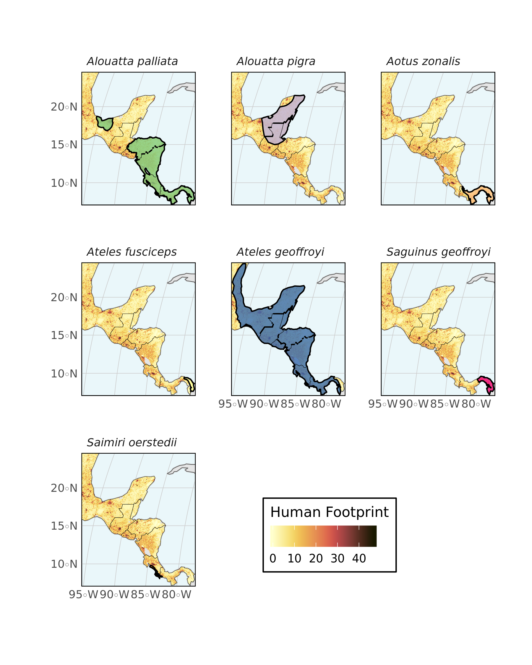
Nice and simple. Any feedback is welcome.