Filter data before reading with awk and R

For a recent project I was working with Fishing Effort data from the Global Fishing Watch (GFW) program. Fishing Effort information is shared by GFW as global spatially-explicit, gridded datasets with fishing vessel locations and whereabouts. These data are open (registration required), and available as daily csv files for each year (since 2012).

A folder with lots of files is a good way to practice iteration, and because the 366 files for 2020 totaled 12 GB in size, this is also a good dataset for trying to pre-process the data before reading it into R.

As I was getting ready to work with this source of data, I was searching for “r filter data before reading” and I found the release post for vroom 1.0.0. The text mentioned how R can work with connections, and this led me to this video by Jim Hester about connections in R. Since R v.1.2.0, we can run system commands from R and have their output available for reading into our workflows. Connections, and in particular those created by the base function pipe, allow us to run shell commands inside other functions and access their results directly.

awk

For working with delimited text files efficiently, the awk console utility is a good option, allowing us to use the AWK semantic analysis language to parse large files without crashing our computers, as we’ll see in the example.

My overall goal was to read the data for the whole year, work out monthly fishing effort, and map it. If we have a year’s worth of data, organized as one file per day with each file following a YYYYMMDD naming scheme, we can:

1 - Get all the file paths in the folder
2 - Group the files into a list element for each month
3 - Read the (29, 30 or 31) files for each month and bind them into a single object
4 - Summarize the values for each cell for each month
5 – Rasterize the results
6 – Plot them with some geographic context and nice colors

Let’s walk through the code.

1 - Get all the file paths in the folder

2 - Group the files into a list element for each month

With functions from purrr and fs, we can get all the file paths in the folder and group the files into a list element for each month like so. If you register and download the 2020 Fishing Effort data (v2, 0.01° resolution), this should be reproducible.

# Load packages (install first if you don't have them)
library(dplyr)              # CRAN v1.0.7 
library(fs)                 # CRAN v1.5.0     
library(sf)                 # CRAN v0.9-8 
library(stringr)            # CRAN v1.4.0 
library(purrr)              # CRAN v0.3.4 
library(ggplot2)            # CRAN v3.3.3 
library(rnaturalearthhires) # [github::ropensci/rnaturalearthhires] v0.2.0 
library(terra)              # CRAN v1.2-10
library(stars)              # [github::r-spatial/stars] v0.5-3 
library(naniar)             # CRAN v0.6.1 
library(readr)              # CRAN v2.0.0   
library(ggfx)               # CRAN v1.0.0
library(scico)              # CRAN v1.2.0
library(vroom)              # [github::r-lib/vroom] v1.5.3.9000

# path to the unzipped daily csvs
setwd("/your-path-here/fleet-daily-csvs-100-v2-2020")

# daily file names
dailies <- dir_ls(type = "file")
# months vector
monthsyr <- sprintf("%02d", 1:12)
# each month's files
monthliesTF <- paste0("-", monthsyr, "-") %>% map(~ str_detect(dailies, .x))

# subset iteratively
monthly_paths <- monthliesTF %>%
  map(~ dailies[.x]) %>%
  set_names(month.abb)

3 - Read the (29, 30 or 31) files for each month and bind them into a single object

The part that was new to me came in the third step of this workflow, when I needed to prefilter each csv file before importing it into R. This is where AWK saved my RAM and well-being. awk parses data line-by-line and doesn’t need to read the whole file into memory to process it. In AWK, each line in a text file is a record (row) and each line is broken up into a sequence of fields (columns/variables). When awk reads a record, it splits the line into fields based on a delimiter (the input field separator), and we can refer to the fields by position using the dollar sign and their index ($1, $2, $3 hold the values of the first, second, and third fields respectively)

In the command line, we write awk commands like this:

awk 'statement' input.file

First we call awk, followed by a statement enclosed in single quotes, then our input file. Inside the statement, goes the {ACTION} to be taken on the records in the input file, enclosed in curly brackets.

To pre-filter csv files before reading them in R, we need a conditional expression to filter the data on the values of some of the columns, and then print them as delimited text which R can consume without issues.

Conditional expressions in the awk statement follow this syntax:

if (conditional-expression)  action

In this case, to filter records by maximum and minimum latitude and longitude, we first figure out which fields hold these values, and then build the conditional statement. I knew from the dataset description that latitude is the second column and longitude the third, so we can use relational (greater than, less than, etc.; >, <, ==, !=) and logical operators (and, or; &&, ||) to specify our filter.

The statement takes this general form

{if (conditional expression) {action} } input.file

To combine more conditions, we enclose each one in brackets and combine them with a logical operator

{if ((condition a) && (condition b)) {action} } input.file

Finally, the complete shell command will include a call to awk and a specification of the delimiter or input field separator using the -F option. In this case, a comma because we are working with csv files.

awk -F ',' '{ if (($2 > 5.89 && $2 < 13.86) && ($3 > -93.51 && $3 < -84.60)) { print } }' input.file

The maximum and minimum lat/long values for this example define a bounding box I drew manually, for waters off the coasts of El Salvador and Nicaragua. The action to take is to {print} the records that meet the conditions.

To do this iteratively for all the paths inside a list, which correspond to days in different months, we define a function that will paste each file path into the awk shell command, which goes inside a pipe call as an argument tovroom::vroom, along with a vector of column names.

# Manual bounding box created with mapedit::drawFeatures()
# xmin: -93.51716 ymin: 5.892904 xmax: -84.60697 ymax: 13.85601

# define fn to prefilter & read
vroomprefilt <- function(inputfile) {
  colsfleet <- c(
    "date", "cell_ll_lat", "cell_ll_lon",
    "flag", "geartype", "hours", "fishing_hours",
    "mmsi_present"
  )
  vroom(pipe(paste("awk -F ',' '{ if (($2 > 5.89 && $2 < 13.86) && ($3 > -93.51 && $3 < -84.60)) { print } }'", inputfile)),
    col_names = colsfleet
  )
}

Now we can iterate through all the months and days, drop the empty tibbles (days with no fishing effort recorded in the area) with discard and a predicate function.

# read and filter all months
allEffort <- map(month.abb, ~ monthly_paths[[.x]]) %>% map_depth(2, vroomprefilt)
# drop empty tibbles
allEffort <- allEffort %>% map(~ discard(.x, ~ nrow(.x) == 0))

4 - Summarize the values for each cell for each month

We are ready to summarize the monthly data for each grid cell. To summarize by month, we can define a function to bind the daily tibbles into a single object for the whole month and then use dplyr to group by lat/long combinations and then summarize the total hours by grid cell. Because the xy data describes the lower left corner of each cell, we can add half the length of a grid cell to each value to shift the coordinates to the cell centers, for rasterization.

# summarize data for each grid cell
get_cellEffort <- function(monthlyEffortdf) {
  monthlydf <- map_df(monthlyEffortdf, bind_rows)
  summ_df <- monthlydf %>%
    mutate(
      cell_ll_lat = cell_ll_lat + 0.005,
      cell_ll_lon = cell_ll_lon + 0.005
    ) %>%
    group_by(cell_ll_lat, cell_ll_lon) %>%
    summarize(
      sum_fishing_hours = sum(fishing_hours, na.rm = T),
      .groups = "drop"
    ) %>%
    naniar::replace_with_na(replace = list(sum_fishing_hours = 0))
}

# summarized data
monthly_xydfs <- map(allEffort, get_cellEffort)

5 – Rasterize the results

To produce raster files for each month, I defined a function that creates a matrix with the xy coordinates and fishing hours, then creates a raster with terra::rast (really fast!), and ultimately coerces the output to a stars object. This was simply personal choice. The spatial data can be used as is or as a SpatRaster.

# rasterize each month's df
rasterizedf <- function(xyzdat) {
  xyzobj <- as.matrix.data.frame(xyzdat[c("cell_ll_lon", "cell_ll_lat", "sum_fishing_hours")])
  fishrast <- terra::rast(x = xyzobj, type = "xyz", crs = "+proj=longlat +ellps=WGS84 +datum=WGS84 +no_defs")
  st_as_stars(fishrast)
}

# raster for each month
monthly_rasters <- map(monthly_xydfs, rasterizedf)
names(monthly_rasters) <- month.abb

6 – Plot the rasters with some geographic context and nice colors

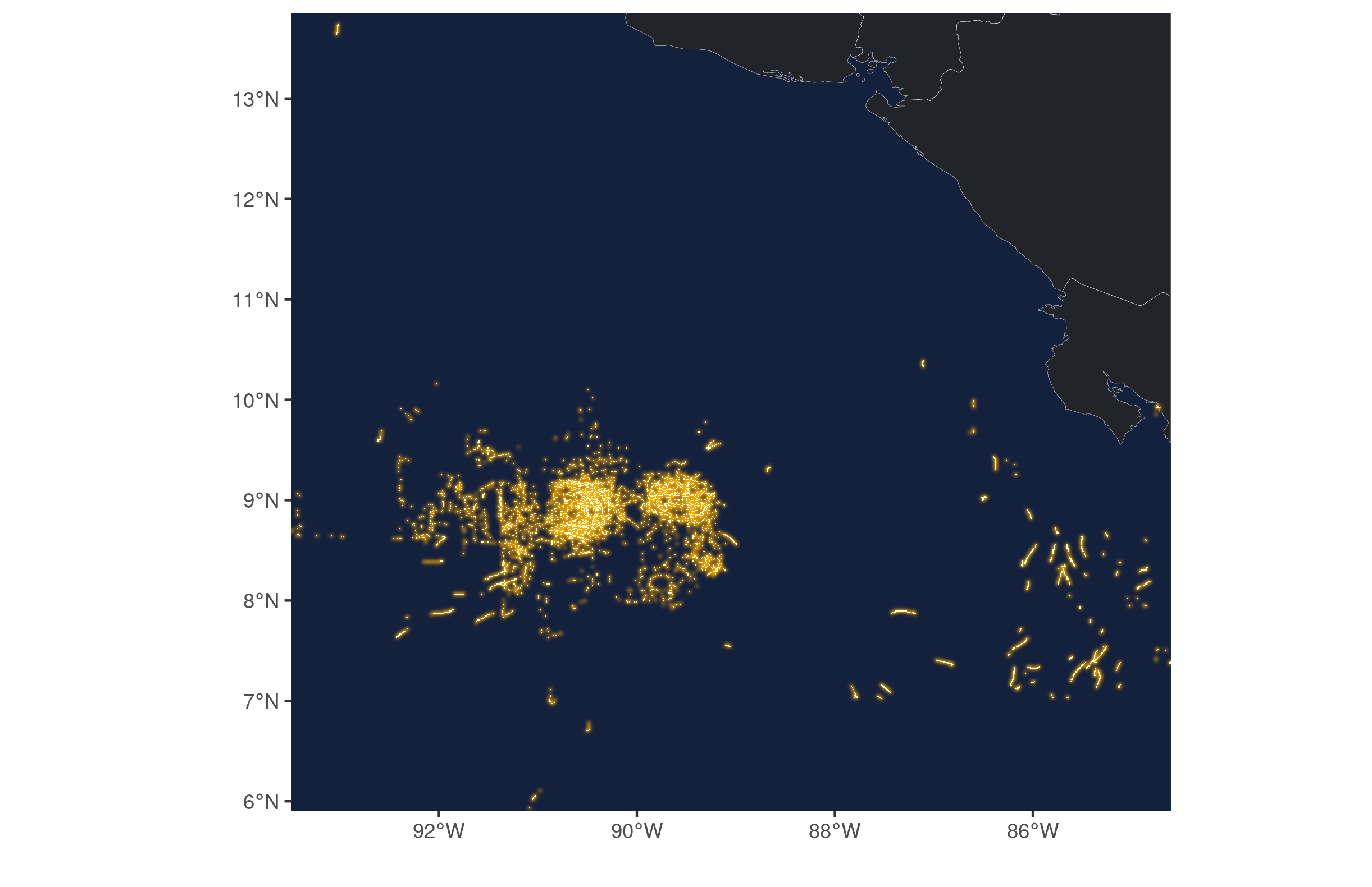
Finally, we can plot the data for one or more of the months. I chose June for no particular reason. For this, we just need a coastline from rnaturalearth and then we can use ggplot to draw the raster and the simple feature coastline. I threw in an outer glow from ggfx for a ‘firefly map’ effect.

# get coastline
library(rnaturalearth) # CRAN v0.1.0
divpol <- ne_countries(scale = 10, country = c("El Salvador", "Nicaragua", "Honduras", "Costa Rica"), returnclass = "sf")
# bounding box
limspat <- st_bbox(st_as_sf(monthly_xydfs[[6]], coords = c("cell_ll_lon", "cell_ll_lat")))
# crop coastline
divpol <- st_crop(divpol, limspat)

# draw
ggplot() +
  geom_sf(data = divpol, size = 0.06, fill = "#212529", color = "white") +
  with_outer_glow(geom_stars(data = monthly_rasters[[6]]), colour = "#ffaa00", sigma = 3, expand = 2) +
  scale_fill_scico(na.value = "transparent", palette =  "lajolla", direction = 1, guide=FALSE) +
  coord_sf(
    expand = FALSE,
    xlim = c(limspat["xmin"], limspat["xmax"]),
    ylim = c(limspat["ymin"], limspat["ymax"])
  ) +
  theme(
    panel.background = element_rect(fill = "#14213d"),
    panel.grid = element_blank()
  )+labs(x="",y="")

For a quick draft, the map looks good.

This post was mainly a way for me to structure my thoughts and learning process on awk, but it really taught me how ‘old-school’ command line tools can work with R. Running some benchmarks early on, I found this crazy difference between reading the files with pre-processing versus using dplyr after reading each one.

expr	mem_alloc	total_time
pre-filtering	247MB	2.76m
read then filter	12GB	4.61m

Timewise, pre-filtering is faster, but the bigger difference is in memory use. 12GB is enough to crash many laptops.

The amount of Real Data Science™ you can do with grep, cut, awk, sed, and perl -pie is truly astounding.
— Stephen Turner (@strnr) August 5, 2021

I only work with big(ish) data occasionally, but will definitely keep using and learning command line tools and their integration with R moving forward.

Here are some good resources I found on awk:

https://www.tim-dennis.com/data/tech/2016/08/09/using-awk-filter-rows.html
https://www.thegeeksearch.com/beginners-guide-to-using-awk-in-shell-scripts/
http://linuxhandouts.com/awk-for-beginners/

Filter data before reading with awk and R

Luis D. Verde Arregoitia

awk

1 - Get all the file paths in the folder

2 - Group the files into a list element for each month

3 - Read the (29, 30 or 31) files for each month and bind them into a single object

4 - Summarize the values for each cell for each month

5 – Rasterize the results

6 – Plot the rasters with some geographic context and nice colors

Share on

You may also enjoy

You ‘tidyr::complete()’ me

What are people commenting about their loaded packages?

Fixing broken and irregular column headers

Waffle charts with svg images