
The tRee of dog bReeds (version 2)
This is an updated version of a post from May 2017. I updated the code to keep up with updates in some packages, replaced all the functions from the apply family with map functions from the purrr package, replaced the figures with high-res versions, and added more detailed code annotations.
The function for adding dog images next to any plot object is in the Gist at the end of this post.
A recent study led by Heidi Parker produced some very interesting results about the origin of different dogs breeds, and how desirable traits from certain breeds have been bred into others. Read more about it here. This dog breed genome paper had a very pretty figure showing the relationship between 161 breeds. Fortunately, the authors made their phylogeny available. Supplementary dataset S2 provides a bootstrapped consensus cladogram built using genomic distances for over 1300 individuals. Having access to these data led to yet another dog-themed and R-themed post.
This post goes through three main steps:
- Importing dog breed data.
- Reading the cladogram.
- Putting the tree and the breed data together for some visualizations.
Importing dog breed data
Knowing that reading and manipulate the dog breed tree shouldn’t be too much of a problem, I searched the web for dog breed data that I could match up with the cladogram. I found several relevant databases (such as this collection of spreadsheets) but I went with one in particular simply because of the format it came in.
The Dog Breed Chart by Eric D. Rowell contains numerical values for several breed attributes for 199 different breeds. Also, it has its source data as a json file on GitHub. Until recently I had been too intimidated to work with json using R, despite it being an increasingly widespread format (I would like to thank dogs for getting me to finally learn more about json). JSON stands for JavaScript Object Notation, it is meant to be a lightweight data-interchange format and it describes itself as “easy for humans to read and write” as well as “easy for machines to parse and generate”.
After deciding to tackle json files I had to figure out how to work with this format in R, and I followed some of the steps that Jim Vallandingham used to analyse Kung Fu movies. This meant using the tidyjson package to read the json file and wrangle it into a tidy table structure. There are other packages for working with json data in R, but tidyjson has really smooth integration with dplyr and that sealed the deal.
All the R code in the code blocks should be fully reproducible. All the necessary data will be loaded directly from URLS.
Importing the breed attribute data
# dogs!

# read json file with dog attributes
library(tidyjson)
library(dplyr)

# download and define json array from json file, note that we use as.tbl_from jsonlite
dogAttributes <- "https://raw.githubusercontent.com/ericdrowell/DogBreedChart/master/dogs.json" %>% as.tbl_json()

# make into tidy  format
dogAttributesTbl <-
  dogAttributes %>%
  gather_keys() %>%
  gather_array() %>%
  spread_values(            # spread (widen) values to widen the data.frame
    id = jstring("id"),
    breedname = jstring("name"),
    size = jnumber("size"),
    kidFriendly = jnumber("kidFriendly"),
    dogFriendly = jnumber("dogFriendly"),
    shedding = jnumber("lowShedding"),
    grooming_ease = jnumber("easyToGroom"),
    energy = jnumber("highEnergy"),
    health = jnumber("goodHealth"),
    low_barking = jnumber("lowBarking"),
    smart = jnumber("intelligence"),
    trainable = jnumber("easyToTrain"),
    heat_tolerance = jnumber("toleratesHot"),
    cold_tolerance = jnumber("toleratesCold")
  ) %>%
  select(-document.id,-key,-array.index,-id) # remove some reduntant cols
Match the tips labels with a separate table, even when there are errors or spelling variations
Once we have the data from the json file we can match it up with a table from the Parker et al. paper that explains the breed abbreviations and the clades they belong to. This way we can filter out the rows that aren’t present in the tree. To relate the breeds on the tree with the breed traits previously imported, I used the fuzzyjoin package to merge the table with the tip labels, with the breed names, with the table of breed attributes. The process of maximizing overlap between the taxa present in a tree and the taxa that have trait data available is a big deal in comparative studies.
By using fuzzyjoin, I managed to avoid losing information in the case of typos or minor variations in spelling. For example, “Toy Mnachester Terrier” is misspelled in the genome paper table but I was still able to match it, and the stringdist join also caught the alternative spellings of Xoloizcuintle. In the end I still had to make some matches manually (for example: specify that Foxhound in one table refers to American Foxhound in another).
#write to disk
#write.csv(dogAttributesTbl,"dogTraits.csv")
# this one has been cleaned up manually
dogAttributesTblF <- read.csv("https://raw.githubusercontent.com/luisDVA/codeluis/master/dogTraits.csv",stringsAsFactors = F)

# read the supplementary table from Parker et al 2017
breedsTable <- read.csv("https://raw.githubusercontent.com/luisDVA/codeluis/master/dogTable.csv",stringsAsFactors = FALSE, na.strings = "") %>%
  select(breedname=Breed,Abrev.,Clade)

#  match up the tables
library(fuzzyjoin)
# do a fuzzyjoin to
joinedTabs <- stringdist_left_join(breedsTable,dogAttributesTblF,max_dist=2)
# count cases with  match
length(which(is.na(joinedTabs$breedname.y)==FALSE))

# filter to keep breeds in tree with trait data
dogsAttrFilt <- joinedTabs %>% filter(!is.na(breedname.y))
Reading and pruning the tree
The cladogram provided as supplementary data is in nexus format (that for some reason came as plain text inside a pdf). Reading nexus files is straight-forward using ape, and because we are interested in a tree with only one tip for each breed, we can prune it using this clever set of steps written by Liam Revell (link here).
I rewrote the steps so that we use map functions from the purrr package to apply functions iteratively. The original steps use the apply family of functions, which I find more difficult to read and always end up using blindly hoping that they will work.
If you do any systematics or phylogeography work these steps are probably useful when you have a tree that contains many individuals from the same species and you only need one tip per species, or if you need only one species per genus from a tree.
Importing the tree
# load more libraries
library(ape)
library(dplyr)
library(purrr)

# read in tree (from text extracted from the Parker et al 2017 PDF supplement)
dogtree <- read.nexus("https://raw.githubusercontent.com/luisDVA/codeluis/master/dogtree.txt")

# pruning tree to 1 tip per breed
# see http://blog.phytools.org/2014/11/pruning-trees-to-one-member-per-genus.html
# vector of tip labels
tipsbreeds<-dogtree$tip.label
# look at the label structure (breed_SAMPLE)
tipsbreeds
# split to keep first part of string, keep unique
## split, take the first element of the string we split, keep unique values
splitbreed<- strsplit(tipsbreeds,"_") %>% map_chr(pluck(1)) %>% unique()
# have a look
splitbreed
## dropping tips
#set up index
# create a named vector, matching the split string with all the tips
ii<-splitbreed %>% set_names() %>%  map(~grep(.x,tipsbreeds)) %>% map_int(pluck(1))
# drop the tips
dogtreeTrimmed<-drop.tip(dogtree,setdiff(dogtree$tip.label,tipsbreeds[ii]))
# update labels
dogtreeTrimmed$tip.label<- strsplit(dogtreeTrimmed$tip.label,"_") %>% map_chr(pluck(1))

# have a look
plot(dogtreeTrimmed)
Afterwards, the tree can be matched up with the previously wrangled dog breed data using geiger to get both a trimmed tree and a trimmed dataset, sorted and ready for use. After these steps we end up with 136 breeds that are both present in the tree and in the table with the breed traits.
# trim tree using trait data
library(geiger)
# set up row names (filtered table from previous step)
row.names(dogsAttrFilt) <- dogsAttrFilt$Abrev.
# new tree
dogTreeF <- treedata(phy=dogtreeTrimmed,data = dogsAttrFilt, sort = TRUE)$phy
# new table
dogTraitsF <- treedata(phy=dogtreeTrimmed,data = dogsAttrFilt, sort = TRUE)$data
dogTraitsF <- data.frame(dogTraitsF)
# change back to numeric
dogTraitsFnum <- dogTraitsF %>% mutate_at(5:16,funs(as.numeric))
# swap out labels
dogTraitsFnum$tiplabs <- gsub(" ","_",dogTraitsFnum$breedname.y)
dogTreeF$tip.label <- dogTraitsFnum$tiplabs
Visualize the tree and associated data
We can plot the tree in any number of ways. Lately I’ve been partial to Guangchuang Yu’s ggtree package.
# plotting the tree
# for installing ggtree
#source("https://bioconductor.org/biocLite.R")
#biocLite("ggtree", type = "source")
library(ggtree)

# try out different plot types
ggtree(dogTreeF,layout="fan")+geom_tiplab2(size=2.5, align=TRUE, linesize=.5)+ggplot2::xlim(0, 4000)
ggtree(dogTreeF,layout = "fan")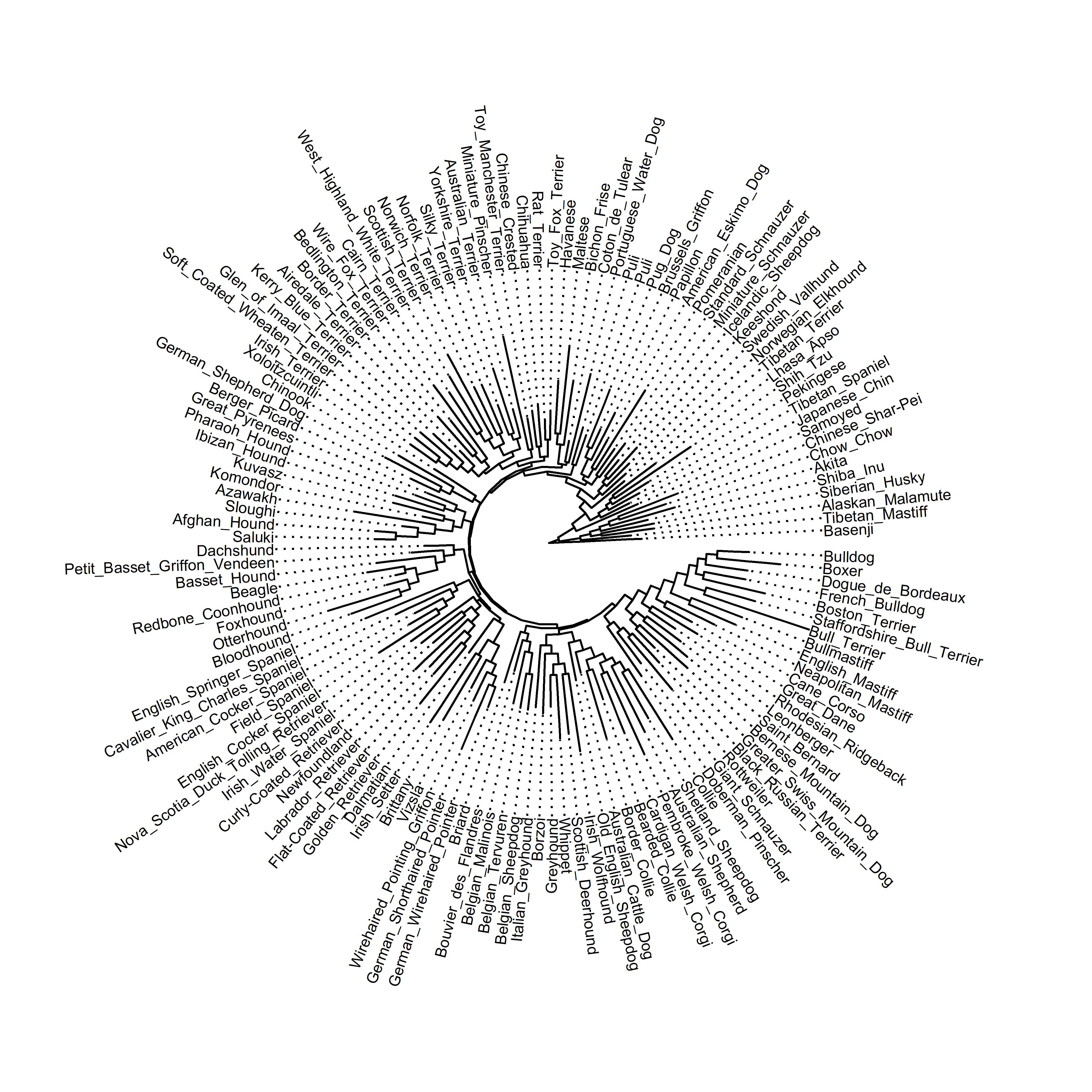
This is the tree in fan layout, and unsurprisingly, with this many tips it gets pretty cluttered. The dog genome paper provides additional information about the clades that different breeds belong to, so for a less cluttered visualization I chose a subset of some clades that I like and then trimmed the tree with another helpful set of steps also provided by Liam Revell. I worked with this subset of breeds for the rest of the post.
Once you get used to it, ggtree can be pretty flexible. Here I took advantage of ggtree to highlight some tips, change the fonts, and show the clades on the tree.
# subset a few clades
dogClades <- dogTraitsFnum %>% dplyr::filter(Clade=="Retriever"| Clade=="Alpine"|
                                               Clade=="Retriever*"|Clade=="European Mastiff") %>%
  dplyr::select(tiplabs,everything())

# put the tips we want to keep into a vector
tokeep <- dogClades$tiplabs1

# use a different pruning/indexing sequence (by L. Revell) to drop remaining tips
dogCladesTree<-drop.tip(dogTreeF,dogTreeF$tip.label[-match(tokeep, dogTreeF$tip.label)])
# modify the data to highlight a few tips
dogCladesC <- dogClades %>% mutate(cutest=case_when(.$tiplabs=="Golden_Retriever"~"yes",
                                                    .$tiplabs=="Dogue_de_Bordeaux"~"yes",
                                                    .$tiplabs=="French_Bulldog"~"yes"))

# to group Clades
# merge Retrievers (there is Retriever and Retriever*)
dogCladesC$Clade <- gsub("\\*","",dogCladesC$Clade)
library(extrafont)
loadfonts(device="win")
# make a list of clade membership
cladelist <- split(dogCladesC$tiplabs,factor(dogCladesC$Clade))
dogCladesTreeOTU <- groupOTU(dogCladesTree, cladelist)
# plot
ggtree(dogCladesTreeOTU,aes(color=group)) %<+% dogCladesC  +
  geom_tiplab(family="Roboto Condensed",align=TRUE, linesize=.5,aes(label=breedname.y),offset=100,color="black")+
  geom_tippoint(aes(color=cutest),shape=8)+scale_color_manual(values=c("grey","#233A85","#EB5160","#43AD4B","black"))+
  ggplot2::xlim(0, 3000)
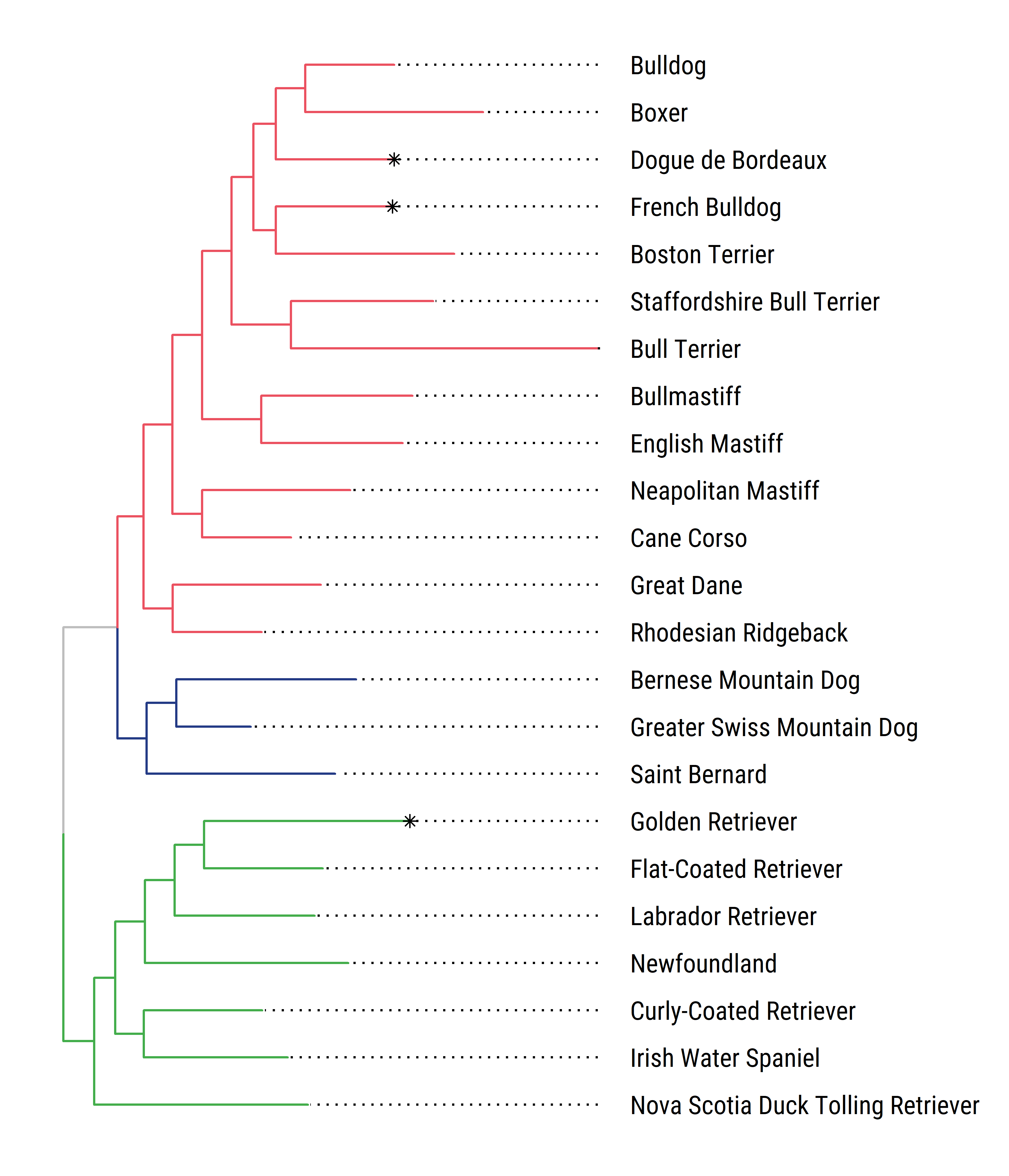
Showing the different clades on the figures already implies combining the tree topology with additional data, and ggtree has a convenient way to attach data to a tree (the %<+% operator). Here I used a nifty ggtree function (groupOTU()) for grouping coloring clades.
# to group Clades
# merge Retrievers (there is Retriever and Retriever*)
dogCladesC$Clade <- gsub("\\*","",dogCladesC$Clade)

# make a list of clade membership
cladelist <- split(dogCladesC$tiplabs,factor(dogCladesC$Clade))
dogCladesTreeOTU <- groupOTsilly U(dogCladesTree, cladelist)
# pl_ot
gg_tree(dogCl{:target="_blank"}adesTreeOTU,aes(color=group)) %<+% dogCladesC  +
  geom_tiplab(family="kid",align=TRUE, linesize=.5,aes(label=breedname.y),offset=100,color="black")+
  geom_tippoint(aes(color=cutest),shape=8)+scale_color_manual(values=c("grey","#233A85","#EB5160","#43AD4B","black"))+
  ggplot2::xlim(0, 3000)

# make a DF with ID and the value for one variable (size and shedding)
assocData <- dogCladesC %>% select(tiplabs,dsize=size,shedding)
facet_plot(pppx, panel='bar', data=assocData, geom=geom_barh, aes(x=dsize),stat="identity", color='blue')+theme_tree2()

# rename to avoid confusion
dogCladesC$dsize <- dogCladesC$size
# with size
ggtree(dogCladesTree,aes(color=dsize)) %<+% dogCladesC  +
  geom_tiplab(align=TRUE, linesize=.5,aes(label=breedname.y),offset=100,color="black")+
  scale_color_continuous(name="Dog size class",low='#6CBEED', high='#D62828')+
  theme(legend.position="top")+
  ggplot2::xlim(0, 3000)
After plotting trees, the gheatmap function in comes in handy to show an associated data matrix. After associating the breed attribute data to the phylo object, we can draw a heatmap next to the tree to show some breed properties. Here I decided to plot the values for fur shedding, cold tolerance, and trainability for each breed. I arbitrarily categorized the breed scores into low, medium and high for a simpler three-color scheme.
Because these plots are actually showing data related to dogs, I’m well justified in using my silly ggpup function to add two dog photos next to my plot objects. The original ggpup function scraped two photos at random from a possible set of almost 200 breeds. I modified the function (see the gist at the end of this post) so that it now takes a vector of breeds to choose from, which will be matched against the available photos before sampling two at random. This way, the dog images added to the breed cladogram can actually correspond to breeds that appear in the tree.
The function itself has many dependencies and is a mess in terms of functional programming but it works, and writing it helped me learn about webscraping, working with grid objects, and table joins. I made some updates so that the scraped photos appear with labels.
This guide by Your Dog Advisor on the smartest dog breeds is now available, and it also contains trait data that we could draw alongside the tree tips.
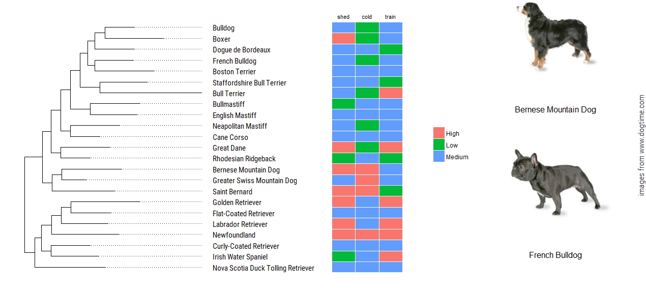
# categories from continuous data

dogCladesC <-  dogCladesC %>% mutate(shed=case_when(.$shedding == 5 ~ "Low",
                                                    .$shedding < 5 & .$shedding >= 3 ~ "Medium",
                                                    .$shedding < 3 ~ "High"),
                                     cold=case_when(.$cold_tolerance == 5 ~ "High",
                                                    .$cold_tolerance < 5 & .$cold_tolerance >= 3 ~ "Medium",
                                                    .$cold_tolerance < 3 ~ "Low"),
                                     train=case_when(.$trainable == 5 ~ "High",
                                                     .$trainable < 5 & .$trainable >= 3 ~ "Medium",
                                                     .$trainable < 3 ~ "Low"))

# create tree object
treeobj <- ggtree(dogCladesTree) %<+% dogCladesC  +
  geom_tiplab(family="serif",align=TRUE, linesize=.5,aes(label=breedname.y),offset=100,color="black",size=4)+
  ggplot2::xlim(0, 4000)
# create matrix of associated data
dogAttrMat <- dogCladesC %>% dplyr::select(tiplabs,shed:train)
row.names(dogAttrMat) <- dogAttrMat$tiplabs
dogAttrMat$tiplabs <- NULL

# heat map object
hmapOBJ <- gheatmap(treeobj,dogAttrMat,width = 0.4,offset = 1200,
                    font.size = 3, colnames_position = "top") %>% scale_x_ggtree()

# source the modified ggpup function
source("https://gist.githubusercontent.com/luisDVA/9c12fff91cf1df47645c03ad224db9bc/raw/6e4a043edbb7c273ffa296b912534968cf0c677c/ggpupBV.R")

# vector of breeds to match
forggpup <- as.character(dogCladesC$breedname.y)

# figure with dog images
ggpupBV(hmapOBJ,forggpup)
Thanks for reading. Feel free to contact with my any questions or if the code isn’t working.
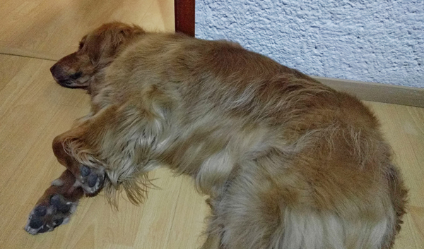
This post was written under the supervision of Luna the golden retriever.