
The tRee of dog bReeds
The function for adding dog images next to any plot object is in the Gist at the end of this post.
This recent study led by Heidi Parker produced some enlightening results about the origin of different dogs, and how desirable traits from certain breeds have been bred into others. Read more about it here. This dog breed genome paper had a pretty figure showing the relationship between 161 breeds, and straight away I checked to see if the authors had shared the tree. Fortunately, they did. Supplementary dataset S2 provides a bootstrapped consensus cladogram built using genomic distances for over 1300 individuals. Having access to these data led to what is now my third consecutive dog-themed and R-themed post.
This post goes through three main steps:
- Importing dog breed data.
- Reading the cladogram.
- Putting the tree and the breed data together for some visualizations.
Importing dog breed data
Knowing that reading and manipulate the dog breed tree shouldn’t be too much of a problem, I started searching the web for dog breed data that I could match up with the cladogram. I found several relevant databases (such as this collection of spreadsheets) but I went with one in particular simply because of the format it came in.
The Dog Breed Chart by Eric D. Rowell contains numerical values for several breed attributes for 199 different breeds. Also, it has its source data as a json file on GitHub. Until now I had been too intimidated to mess with json using R, despite it being an increasingly widespread format (I’d like to thank dogs for getting me to finally learn more about json). JSON stands for JavaScript Object Notation, it is meant to be a lightweight data-interchange format and it describes itself as “easy for humans to read and write” as well as “easy for machines to parse and generate”.
After deciding to tackle json files I had to figure out how to work with this format in R, and once again I followed some of the steps that Jim Vallandingham used to analyse Kung Fu movies. This meant using the tidyjson package to read the json file and wrangle it into a tidy table structure. There are other packages for working with json data in R, but tidyjson has really smooth integration with dplyr and that sealed the deal.
All the R code in the code blocks should be fully reproducible, and the only file that needs to be
downloaded locally first is the json file (I think the read_json function breaks with URL file paths - I’ve already created an issue).
Update - 20/06/2017: It looks like the read_json function will be revamped soon. In the meantime, jsonlite::fromJSON works fine with URL sources, and that is what as.tbl_json calls behind the scenes. See the issue comments here.
The updated code will download the json file directly from a URL, without the need for saving it to your workspace beforehand.
Importing the breed attribute data
# dogs!

# read json file with dog attributes
library(tidyjson)
library(dplyr)

# download and define json array from json file
dogAttributes <- "https://raw.githubusercontent.com/ericdrowell/DogBreedChart/master/dogs.json" %>% as.tbl_json()

# make into tidy  format
dogAttributesTbl <-
  dogAttributes %>%
  gather_keys() %>%
  gather_array() %>%
  spread_values(            # spread (widen) values to widen the data.frame
    id = jstring("id"),
    breedname = jstring("name"),
    size = jnumber("size"),
    kidFriendly = jnumber("kidFriendly"),
    dogFriendly = jnumber("dogFriendly"),
    shedding = jnumber("lowShedding"),
    grooming_ease = jnumber("easyToGroom"),
    energy = jnumber("highEnergy"),
    health = jnumber("goodHealth"),
    low_barking = jnumber("lowBarking"),
    smart = jnumber("intelligence"),
    trainable = jnumber("easyToTrain"),
    heat_tolerance = jnumber("toleratesHot"),
    cold_tolerance = jnumber("toleratesCold")
  ) %>%
  select(-document.id,-key,-array.index,-id) # remove some reduntant cols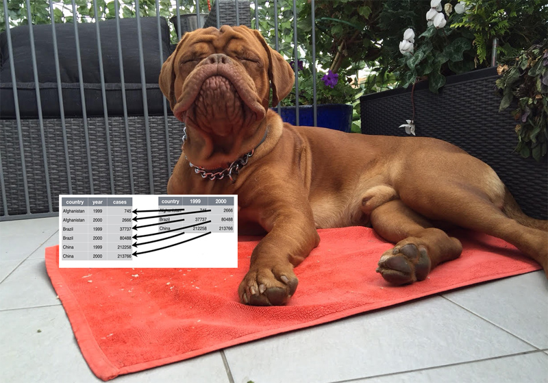
Once we have the data from the json file we can match it up with a table from the Parker et al. paper that explains the breed abbreviations and the clades they belong to. This way we can filter out the rows that aren’t present in the tree. To relate the breeds on the tree with the breed traits previously imported, I used the fuzzyjoin package to merge the table with the tip labels, with the breed names, with the table of breed attributes. The process of maximizing overlap between the taxa present in a tree and the taxa that have trait data available is a big deal in comparative studies. By using fuzzyjoin, I managed to avoid losing information in the case of typos or minor variations in spelling. For example, “Toy Mnachester Terrier” is misspelled in the genome paper table but I was still able to match it, and the stringdist join also caught the alternative spellings of Xoloizcuintle. In the end I still had to make some matches manually (for example: change Pug to Pug Dog and specify that Foxhound in one table refers to American Foxhound in another).
#write to disk
#write.csv(dogAttributesTbl,"dogTraits.csv")
# this one has been cleaned up manually
dogAttributesTblF <- read.csv("https://raw.githubusercontent.com/luisDVA/codeluis/master/dogTraits.csv",stringsAsFactors = F)

# read the supplementary table from Parker et al 2017
breedsTable <- read.csv("https://raw.githubusercontent.com/luisDVA/codeluis/master/dogTable.csv",stringsAsFactors = FALSE, na.strings = "") %>%
  select(breedname=Breed,Abrev.,Clade)

#  match up the tables
library(fuzzyjoin)
# do a fuzzyjoin to
joinedTabs <- stringdist_left_join(breedsTable,dogAttributesTblF,max_dist=2)
# count cases with  match
length(which(is.na(joinedTabs$breedname.y)==FALSE))

# filter to keep breeds in tree with trait data
dogsAttrFilt <- joinedTabs %>% filter(!is.na(breedname.y))
Reading and pruning the tree
The cladogram provided as supplementary data is in nexus format (that for some reason came as plain text inside a pdf). Reading nexus files is straight-forward using ape, and because we are interested in a tree with only one tip for each breed, we can prune it using this clever set of steps written by Liam Revell (link here).
Importing the tree
# read the tree
library(ape)
#read in tree (from text extracted from the Parker et al 2017 PDF supplement)
dogtree <- read.nexus("https://raw.githubusercontent.com/luisDVA/codeluis/master/dogtree.txt")

# pruning tree to 1 tip per breed
# see http://blog.phytools.org/2014/11/pruning-trees-to-one-member-per-genus.html
# vector of tip labels
tipsbreeds<-dogtree$tip.label
# look at the label structure (breed_SAMPLE)
tipsbreeds
# split to keep first part of string, keep unique
splitbreed<-unique(sapply(strsplit(tipsbreeds,"_"),function(x) x[1]))
## dropping tips
#set up index
ii<-sapply(splitbreed,function(x,y) grep(x,y)[1],y=tipsbreeds)
# drop the tips
dogtreeTrimmed<-drop.tip(dogtree,setdiff(dogtree$tip.label,tipsbreeds[ii]))
# update labels
dogtreeTrimmed$tip.label<-sapply(strsplit(dogtreeTrimmed$tip.label,"_"),function(x) x[1])
Afterwards, the tree can be matched up with the previously wrangled dog breed data using geiger to get both a trimmed tree and a trimmed dataset, sorted and ready for use. After these steps we end up with 136 breeds that are both present in the tree and in the table with the breed traits.
# trim tree using trait data
library(geiger)
# set up row names (filtered table from previous step)
row.names(dogsAttrFilt) <- dogsAttrFilt$Abrev.
# new tree
dogTreeF <- treedata(phy=dogtreeTrimmed,data = dogsAttrFilt, sort = TRUE)$phy
# new table
dogTraitsF <- treedata(phy=dogtreeTrimmed,data = dogsAttrFilt, sort = TRUE)$data
dogTraitsF <- data.frame(dogTraitsF)
# change back to numeric
dogTraitsFnum <- dogTraitsF %>% mutate_at(5:16,funs(as.numeric))
# swap out labels
dogTraitsFnum$tiplabs <- gsub(" ","_",dogTraitsFnum$breedname.y)
dogTreeF$tip.label <- dogTraitsFnum$tiplabs
Visualize the tree and associated data
We can plot the tree in any number of ways. Lately I’ve been partial to Guangchuang Yu’s ggtree package.
# plotting the tree
# for installing ggtree
#source("https://bioconductor.org/biocLite.R")
#biocLite("ggtree", type = "source")
library(ggtree)

# different plot types
gtree(dogTreeF)+geom_tiplab(size=2, align=TRUE, linesize=.5)+ggplot2::xlim(0, 3000)
ggtree(dogTreeF,layout="fan")+geom_tiplab2(size=2.5, align=TRUE, linesize=.5)+ggplot2::xlim(0, 4000)
ggtree(dogTreeF,layout = "fan")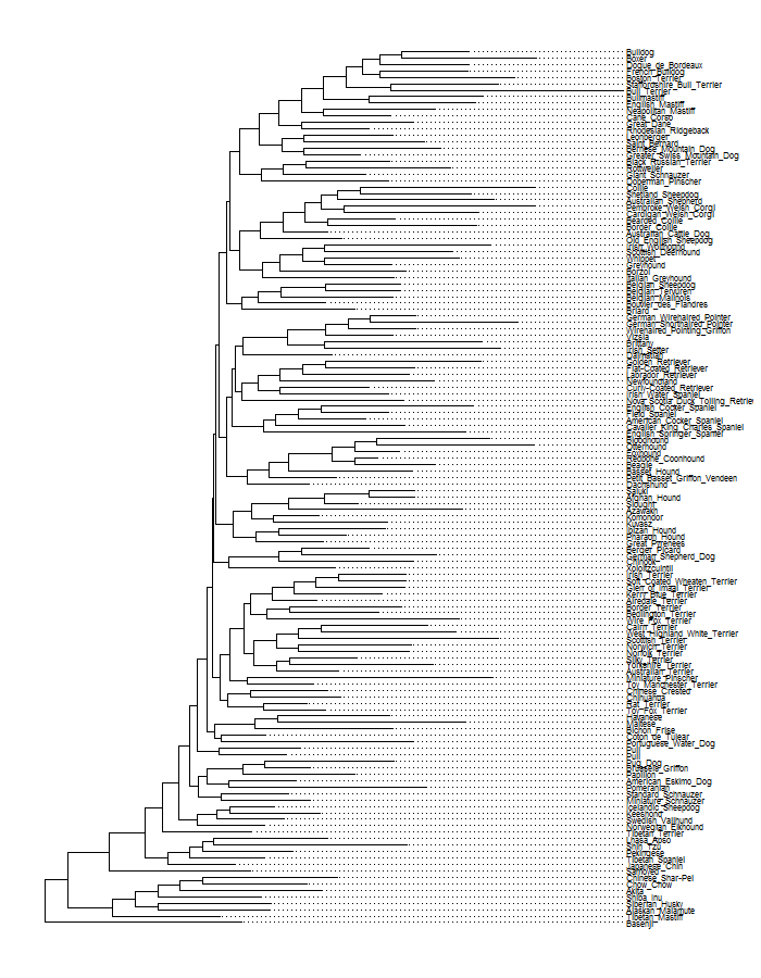
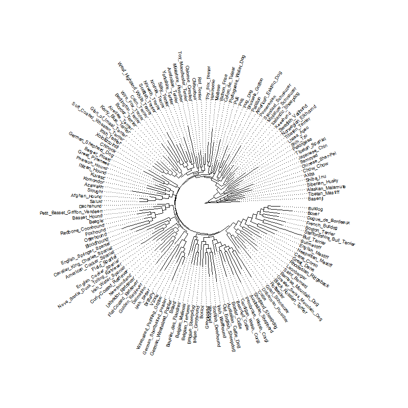
This is the tree in rectangular and fan layout, and unsurprisingly, with this many tips it gets pretty cluttered. The dog genome paper provides additional information about the clades that different breeds belong to, so for a less cluttered visualization I chose a subset of some clades that I like and then trimmed the tree with another helpful set of steps also provided by Liam Revell. I worked with this subset of breeds for the rest of the post.
Once you get used to it, ggtree can be pretty flexible. Here I took advantage of ggtree to highlight some tips, change the fonts, and show the clades on the tree.
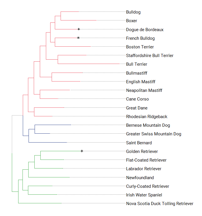
Showing the different clades on the figures already implies combining the tree topology with additional data, and ggtree has a convenient way to attach data to a tree (the %<+% operator).
# subset a few clades
dogClades <- dogTraitsFnum %>% dplyr::filter(Clade=="Retriever"| Clade=="Alpine"|
Clade=="Retriever*"|Clade=="European Mastiff") %>%
dplyr::select(tiplabs,everything())
# put the tips we want to keep into a vector
tokeep <- dogClades$tiplabs
# use a different pruning/indexing sequence (by L. Revell) to drop remaining tips
dogCladesTree<-drop.tip(dogTreeF,dogTreeF$tip.label[-match(tokeep, dogTreeF$tip.label)])
# modify the data to highlight a few tips
dogCladesC <- dogClades %>% mutate(cutest=case_when(.$tiplabs=="Golden_Retriever"~"yes",
.$tiplabs=="Dogue_de_Bordeaux"~"yes",
.$tiplabs=="French_Bulldog"~"yes"))
# plot with extra data
ggtree(dogCladesTree) %<+% dogCladesC +
geom_tiplab(family="serif",align=TRUE, linesize=.5,aes(label=breedname.y),offset=100)+
geom_tippoint(aes(color=cutest),shape=8)+scale_color_manual(values=c("blue", "white"))+
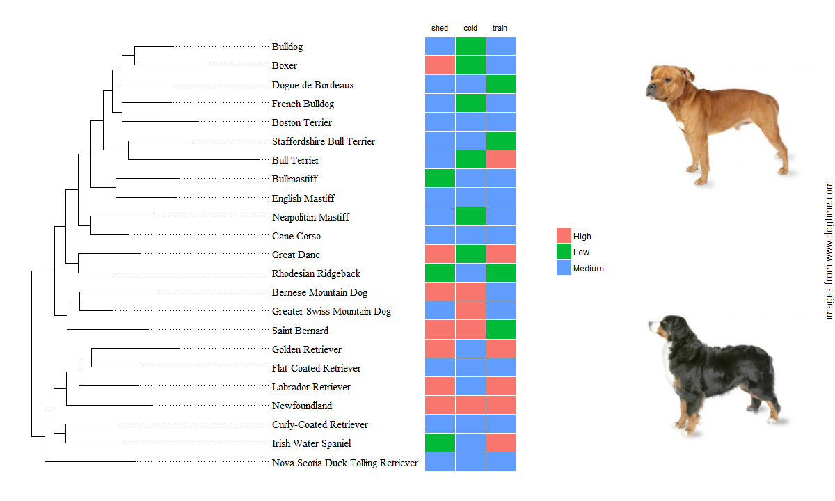
ggplot2::xlim(0, 3000)The breed attributes table contains columns with numerical values for different dog traits, all of them ranging from one to five. I don’t know much about the source of this ratings, but for this post I simply assumed that they represent a coarse continuous variable (instead of an ordinal variable). Just to play around, we can add some of these variables to the tree visualizations. First as continuous values, then as categories.
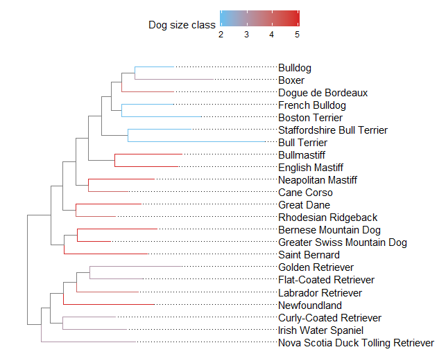
To categorize the ‘continuous’ values, I used case_when and some pretty arbitrary tresholds. After that, the gheatmap function in ggtree comes in handy to show an associated data matrix. Because these plots are actually showing data related to dogs, I’m well justified in using my ggpup function to add two dog photos next to my plot objects. The original ggpup function scraped two photos at random from a possible set of almost 200 breeds. I modified the function (see the gist at the end of this post) so that it now takes a vector of breeds to choose from, which will be matched against the available photos before sampling two at random. This way, the dog images added to the breed cladogram can actually correspond to breeds that appear in the tree.
# to group Clades
# merge Retrievers (there is Retriever and Retriever*)
dogCladesC$Clade <- gsub("\\*","",dogCladesC$Clade)

# make a list of clade membership
cladelist <- split(dogCladesC$tiplabs,factor(dogCladesC$Clade))
dogCladesTreeOTU <- groupOTU(dogCladesTree, cladelist)
# plot
ggtree(dogCladesTreeOTU,aes(color=group)) %<+% dogCladesC  +
  geom_tiplab(family="kid",align=TRUE, linesize=.5,aes(label=breedname.y),offset=100,color="black")+
  geom_tippoint(aes(color=cutest),shape=8)+scale_color_manual(values=c("grey","#233A85","#EB5160","#43AD4B","black"))+
  ggplot2::xlim(0, 3000)

# make a DF with ID and the value for one variable (size and shedding)
assocData <- dogCladesC %>% select(tiplabs,dsize=size,shedding)
facet_plot(pppx, panel='bar', data=assocData, geom=geom_barh, aes(x=dsize),stat="identity", color='blue')+theme_tree2()

# rename to avoid confusion
dogCladesC$dsize <- dogCladesC$size
# with size
ggtree(dogCladesTree,aes(color=dsize)) %<+% dogCladesC  +
  geom_tiplab(align=TRUE, linesize=.5,aes(label=breedname.y),offset=100,color="black")+
  scale_color_continuous(name="Dog size class",low='#6CBEED', high='#D62828')+
  theme(legend.position="top")+
  ggplot2::xlim(0, 3000)

# categories from continuous data

dogCladesC <-  dogCladesC %>% mutate(shed=case_when(.$shedding == 5 ~ "Low",
                                                    .$shedding < 5 & .$shedding >= 3 ~ "Medium",
                                                    .$shedding < 3 ~ "High"),
                                     cold=case_when(.$cold_tolerance == 5 ~ "High",
                                                    .$cold_tolerance < 5 & .$cold_tolerance >= 3 ~ "Medium",
                                                    .$cold_tolerance < 3 ~ "Low"),
                                     train=case_when(.$trainable == 5 ~ "High",
                                                     .$trainable < 5 & .$trainable >= 3 ~ "Medium",
                                                     .$trainable < 3 ~ "Low"))

# create tree object
treeobj <- ggtree(dogCladesTree) %<+% dogCladesC  +
  geom_tiplab(family="serif",align=TRUE, linesize=.5,aes(label=breedname.y),offset=100,color="black",size=4)+
  ggplot2::xlim(0, 4000)
# create matrix of associated data
dogAttrMat <- dogCladesC %>% dplyr::select(tiplabs,shed:train)
row.names(dogAttrMat) <- dogAttrMat$tiplabs
dogAttrMat$tiplabs <- NULL

# heat map object
hmapOBJ <- gheatmap(treeobj,dogAttrMat,width = 0.4,offset = 1200,
                    font.size = 3, colnames_position = "top") %>% scale_x_ggtree()

# source the modified ggpup function
source("https://gist.githubusercontent.com/luisDVA/101374d9d6b569d887a1a2c7654cd3a4/raw/a98641561afbe7efa4d8ed6d7e1aac6f62abe2e2/ggpup.R")

# vector of breeds to match
forggpup <- as.character(dogCladesC$breedname.y)

# figure with dog images
ggpupBV(hmapOBJ,forggpup)
Thanks for reading. Feel free to contact with my any questions or if the code isn’t working.
This post was written under the supervision of Luna the golden retriever.