
Animate your data wrangling
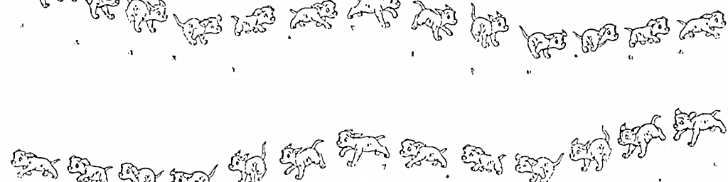
Yesterday I tweeted this gif showing what we can do about non-data grouping rows embedded in the data rectangle using the ‘unheadr’ package (we can and we should put them into their own variable in a tidier way). Please ignore the typo in the tweet.
manage to animate what we can do about non-data grouping rows embedded in the data rectangle using my silly little #rstats package 📦https://t.co/QP1X6ORtH8https://t.co/zJfVslUedN pic.twitter.com/KnAYdSAmc7
— Luis D. Verde (@LuisDVerde) August 12, 2018
There was some interest in the code behind the animation, and I wanted to share it anyway because it’s based on actual data and I think that’s pretty cool.
This is all made possible thanks to Thomas Lin Pedersen’s ‘gganimate’ package, a cool usecase with geom_tile() plots by @mikefc, and this post by David Robison where he melts a table into long format with indices for each row and column and a variable holding the value for each cell.
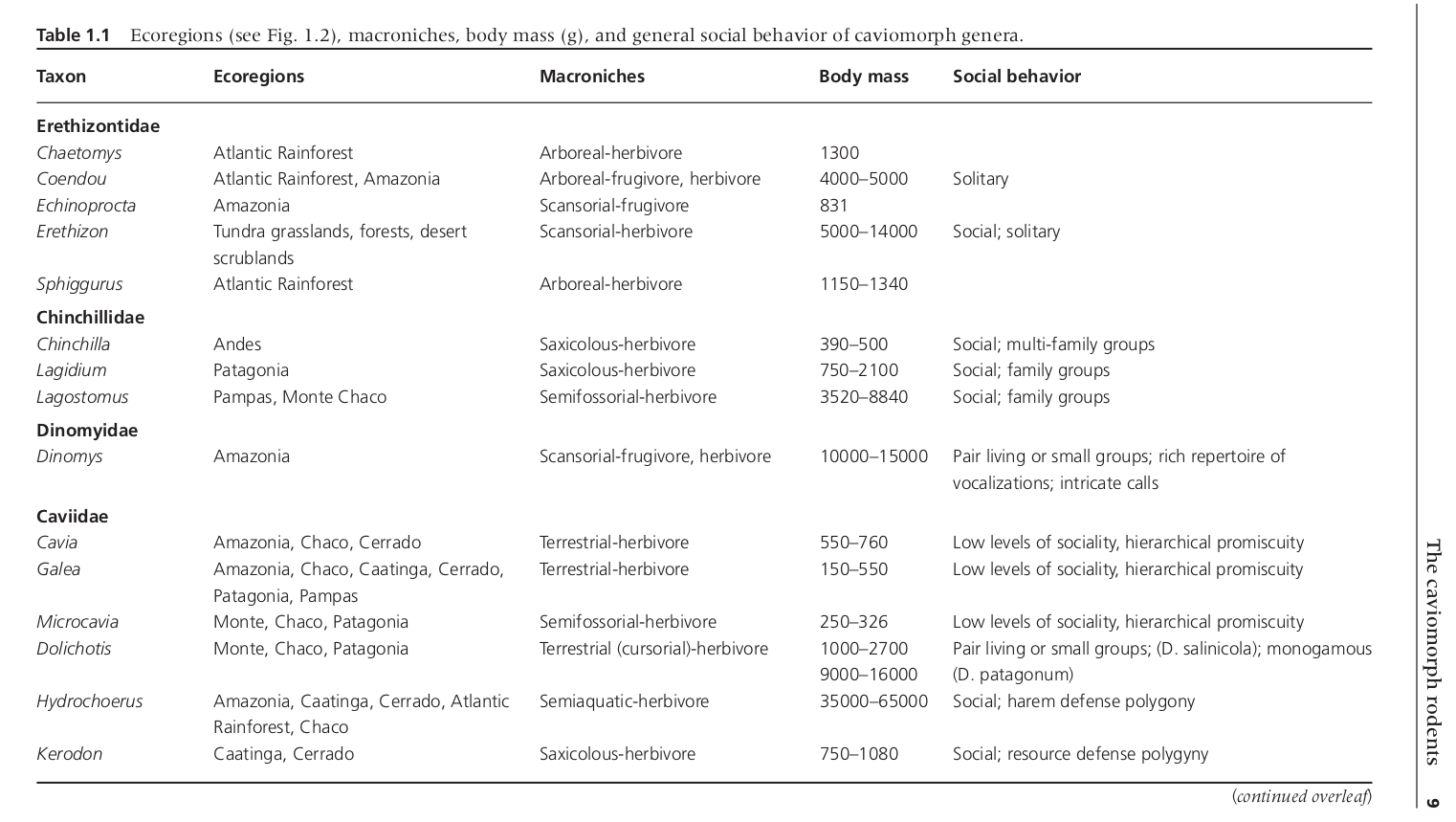
We can use real data from this table, originally from a book chapter about rodent sociobiology by Ojeda et al. (2016). I had a PDF version of the chapter, and I got the data into R following this post by Bob Rudis. I highly recommend ‘pdftools’ and ‘readr’ for importing PDF tables.
The book cover.
The first few lines of the table looked like this, and for this demo we can just set up the data directly as a tibble.
Setting up the data.
# load libraries
library(tibble)
library(dplyr)
library(unheadr)
library(purrr)
library(gganimate)
# tibble
table1 <- tribble(
  ~Taxon,                                     ~Ecoregions,                      ~Macroniches,    ~Body_mass,
  "Erethizontidae",                                              NA,                                NA,            NA,
  "Chaetomys",                           "Atlantic Rainforest",              "Arboreal-herbivore",        "1300",
  "Coendou",                 "Atlantic Rainforest, Amazonia",   "Arboreal-frugivore, herbivore",   "4000–5000",
  "Echinoprocta",                                      "Amazonia",            "Scansorial-frugivore",         "831",
  "Erethizon", "Tundra grasslands, forests, desert scrublands",            "Scansorial-herbivore",  "5000–14000",
  "Sphiggurus",                           "Atlantic Rainforest",              "Arboreal-herbivore",   "1150–1340",
  "Chinchillidae",                                              NA,                                NA,            NA,
  "Chinchilla",                                         "Andes",            "Saxicolous-herbivore",     "390–500",
  "Lagidium",                                     "Patagonia",            "Saxicolous-herbivore",    "750–2100",
  "Lagostomus",                           "Pampas, Monte Chaco",         "Semifossorial-herbivore",   "3520–8840",
  "Dinomyidae",                                              NA,                                NA,            NA,
  "Dinomys",                                      "Amazonia", "Scansorial-frugivore, herbivore", "10000–15000",
  "Caviidae",                                              NA,                                NA,            NA,
  "Cavia",                      "Amazonia, Chaco, Cerrado",           "Terrestrial-herbivore",     "550–760"
)
There are grouping values for the taxonomic families that the different genera belong to, and these are interspersed within the taxon variable. All taxonomic families end with “dae”, so we can match this with regex easily. Install ‘unheadr’ from GitHub before proceeding.
table1_tidy <- table1 %>% untangle2("dae$",Taxon,Family) Once we have the original and ‘untangled’ version of the table, we define a function (inspired by @drob) to melt the data and apply it to each one.
longDat <- function(x){
  x %>%
    setNames(seq_len(ncol(x))) %>%
    mutate(row = row_number()) %>%
    tidyr::gather(column, value, -row) %>%
    mutate(column = as.integer(column)) %>%
    ungroup() %>%
    arrange(column, row)
}

long_tables <- map(list(table1,table1_tidy),longDat)
Next we add two additional variables to the long-form tables, one for mapping fill colors and a label for facets (either in time or in space!).
tab1_long_og <- long_tables[[1]] %>%
  mutate(header=as.character(str_detect(value,"dae$"))) %>%
  group_by(header) %>% mutate(headerid = row_number()) %>%
  mutate(celltype=
           case_when(
             header=="TRUE"~ as.character(headerid),
             is.na(header)  ~ NA_character_,
             TRUE~"data"
           )) %>% ungroup() %>% mutate(tstep="a")

tab1_long_untangled <- long_tables[[2]] %>%
  mutate(header=as.character(str_detect(value,"dae$"))) %>%
  filter(header==TRUE) %>% distinct(value) %>% mutate(gpid=as.character(1:n())) %>%
  right_join(long_tables[[2]]) %>% mutate(celltype=if_else(is.na(gpid),"data",gpid)) %>%
  mutate(tstep="b")
After binding the two together, we can plot the tables as geom_tiles and use the ‘tstep’ variable to view them either side by side, or one after the other.
longTabs_both <- bind_rows(tab1_long_og,tab1_long_untangled)
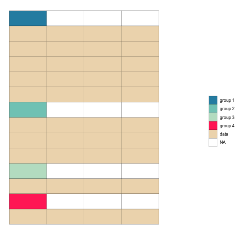
ggplot(longTabs_both,aes(column, -row, fill = celltype)) +
geom_tile(color = "black") +
theme_void()+facet_wrap(~tstep)+
scale_fill_manual(values=c("#247ba0","#70c1b3","#b2dbbf","#ff1654","#ead2ac","gray"),
name="",
labels=c(c(paste("group",seq(1:4)),"data","NA")))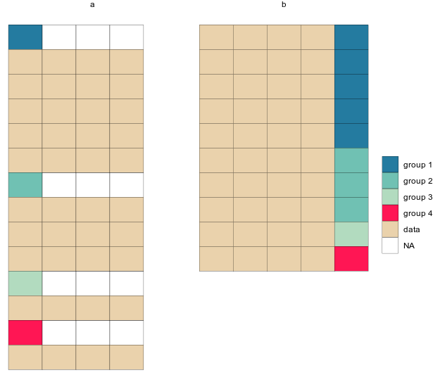
For now, ‘gganimate’ is only available on GitHub. Once we have installed it, ‘transition_states’ does all the magic.
ut_animation <-
  ggplot(longTabs_both,aes(column, -row, fill = celltype)) +
  geom_tile(color = "black")+
  theme_void()+
  scale_fill_manual(values=c("#247ba0","#70c1b3","#b2dbbf","#ff1654","#ead2ac","gray"),
                   name="",
                   labels=c(c(paste("group",seq(1:4)),"data","NA")))+
  transition_states(
    states            = tstep, # variable in data
    transition_length = 1,   # all states display for 1 time unit
    state_length      = 1    # all transitions take 1 time unit
  ) +
  enter_fade() +             # How new blocks appear
  exit_fade() +              # How blocks disappear
  ease_aes('sine-in-out')
Check it out!
Once the animation is rendered we can save it to disk using anim_save().
This approach seems like a good way to animate various types of common steps in data munging, and it should work nicely to illustrate how several ‘dplyr’ or ‘tidyr’ verbs work. I’ll make more animations in the near future.
Thanks for reading!