
Versión en español aquí
A while back, a colleague from Cuba contacted me seeking help with making species richness maps for plants. I had written about species richness maps in R before, but only when working with point occurrence data or species range polygons. In their case, the task was to reclassify and sum a bunch of MaxEnt models to create a species richness layer.
I tried to point them to existing tutorials, but didn’t find any recent ones with good exposition, so here we are. I haven’t run my own SDMs in years, but as far as I know, this should still be the overall process.
-
Run a distribution model (repeat for n species)
-
Pick a threshold and reclassify each species’ raster layer with continuous values of suitability or probability of occurrence into binary presence/absence values.
-
Sum the reclassified layers to count the total species richness for each cell
Disclaimer: I don’t know how others are doing this recently (I suspect with QGIS or ESRI software).
Thanks to all the ongoing development happening with spatial methods in R, a stars + sf + tidyverse approach to raster calculations and plotting is now possible, and below is my take on it.
Proof of concept
Let’s start with a proof of concept. Before working with real data I wanted to see if the approach I cooked up works. For this, we’ll create toy rasters with random suitability values.
The function below creates a 4x5 matrix with random values, converted to a stars object with a silly name created by ids::adjective_animal.
# load libraries
library(stars) # CRAN v0.5-1
library(sf) # CRAN v0.9-7
library(fs) # CRAN v1.5.0
library(rnaturalearth) # CRAN v0.1.0
library(dplyr) # CRAN v1.0.4
library(purrr) # CRAN v0.3.4
library(ggplot2) # CRAN v3.3.3
library(ids) # CRAN v1.0.1
library(tidyr) # CRAN v1.1.2
library(scico) # CRAN v1.2.0
library(patchwork) # CRAN v1.1.1
library(ggthemes) # CRAN v4.2.0
library(colormap) # CRAN v0.1.4
library(extrafont) # CRAN v0.17
library(ggfx) # [github::thomasp85/ggfx] v0.0.0.9000

# set a seed for reproducibility
set.seed(20)

# matrix to stars
make_toy_raster <- function(m) {
  m <- matrix(sample(seq(0, 100, 1), 20, replace = TRUE), nrow = 5, ncol = 4)
  dim(m) <- c(x = 5, y = 4) # named dim
  s <- st_as_stars(m)
  names(s) <- ids::adjective_animal(1)
  s
}
We’ll run this 8 times with purrr::rerun, stack the objects with c(), then combine them with merge().
# make 8 toy rasters
toy_data <- rerun(8, make_toy_raster(m))
allsps <- reduce(toy_data, c)
allspsmg <- merge(allsps)
stars objects have attributes and dimensions, which are the cell values, and the metadata for the dimensions in the array, respectively. We can set these names by passing character vectors to setNames (for attributes) and st_set_dimensions (for the xy coordinates and the species, in this case).
# informative names for the cell values and the dimensions metadata
allspsmg <- setNames(allspsmg, "prob") %>% st_set_dimensions(names = c("x", "y", "sp"))
Printing the object gives us this:
> allspsmg
stars object with 3 dimensions and 1 attribute
attribute(s):
     prob
 Min.   :  1.00
 1st Qu.: 24.00
 Median : 51.00
 Mean   : 50.11
 3rd Qu.: 74.00
 Max.   :100.00
dimension(s):
   from to offset delta refsys point
x     1  5      0     1     NA FALSE
y     1  4      0     1     NA FALSE
sp    1  8     NA    NA     NA    NA
                                             values x/y
x                                              NULL [x]
y                                              NULL [y]
sp inflatable_partridge,...,institutional_pronghorn
This set of layers is ready for plotting with ggplot2
# plot the toy rasters
ggplot() +
  geom_stars(data = allspsmg) +
  coord_equal() +
  scale_fill_scico(palette = "davos", direction = -1, name = "Habitat suitability") +
  theme_bw() +
  facet_wrap("sp", ncol = 4) +
  labs(x = "", y = "") +
  theme(legend.position = "bottom") +
  labs(title = "")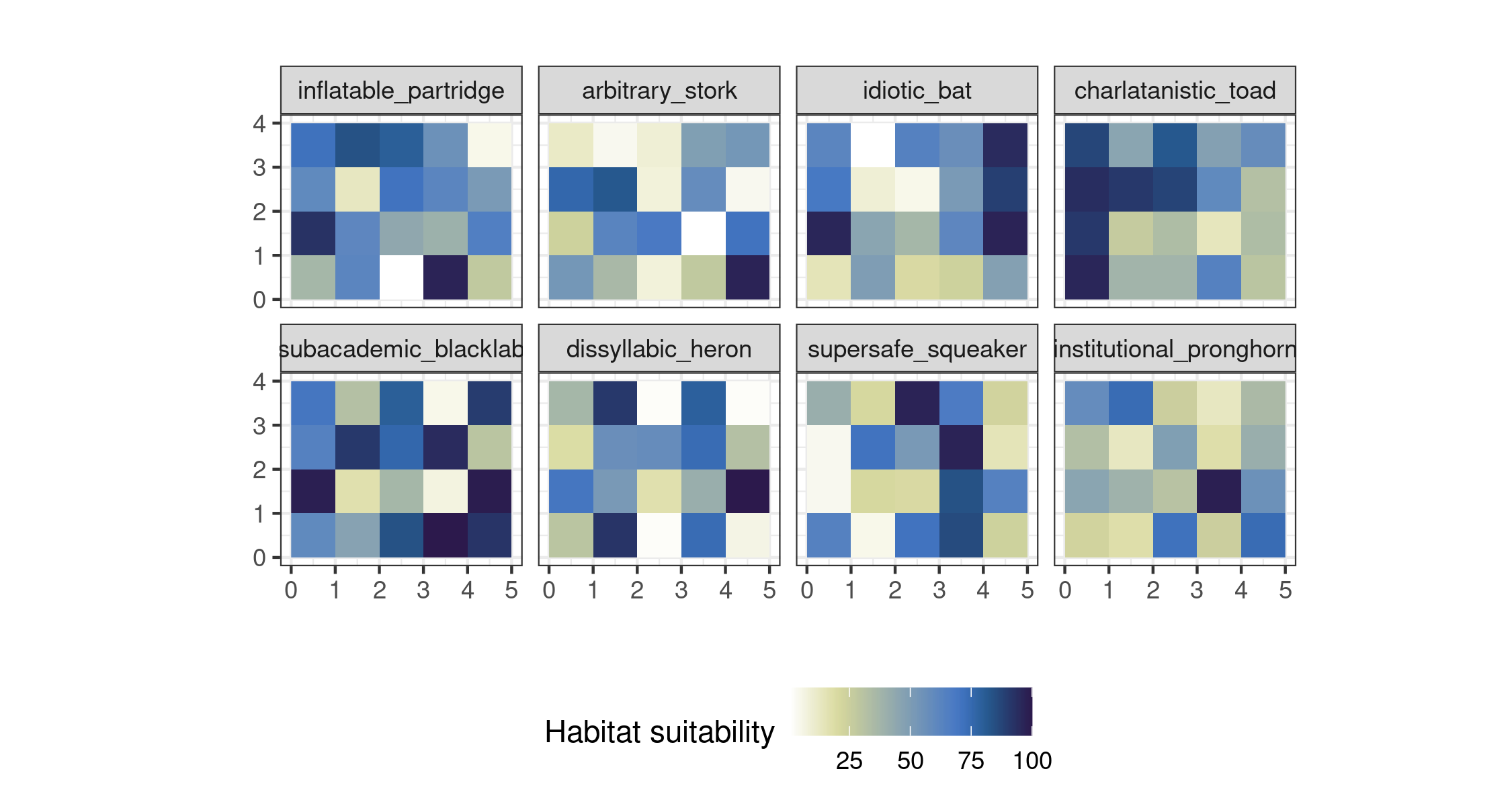
To reclassify all of the arrays, we can use tidyverse methods. Here we consider every cell value >70 as present (1) and <70 as absent (0). It’s very cool how we can use dplyr verbs directly on the stars attributes.
# reclassify to binary
allspRC <-
  allspsmg %>%
  mutate(presence = case_when(
    prob > 70 ~ 1,
    TRUE ~ 0
  )) %>%
  select(presence)
We can also plot the reclassified arrays as a faceted ggplot2 plot.
ggplot() +
  geom_stars(data = allspRC) +
  coord_equal() +
  scico::scale_fill_scico(palette = "davos", direction = -1, name = "Habitat suitability", guide = FALSE) +
  theme_bw() +
  facet_wrap("sp", ncol = 4) +
  labs(x = "", y = "") +
  labs(title = "Reclassified presence/absence in grid cells")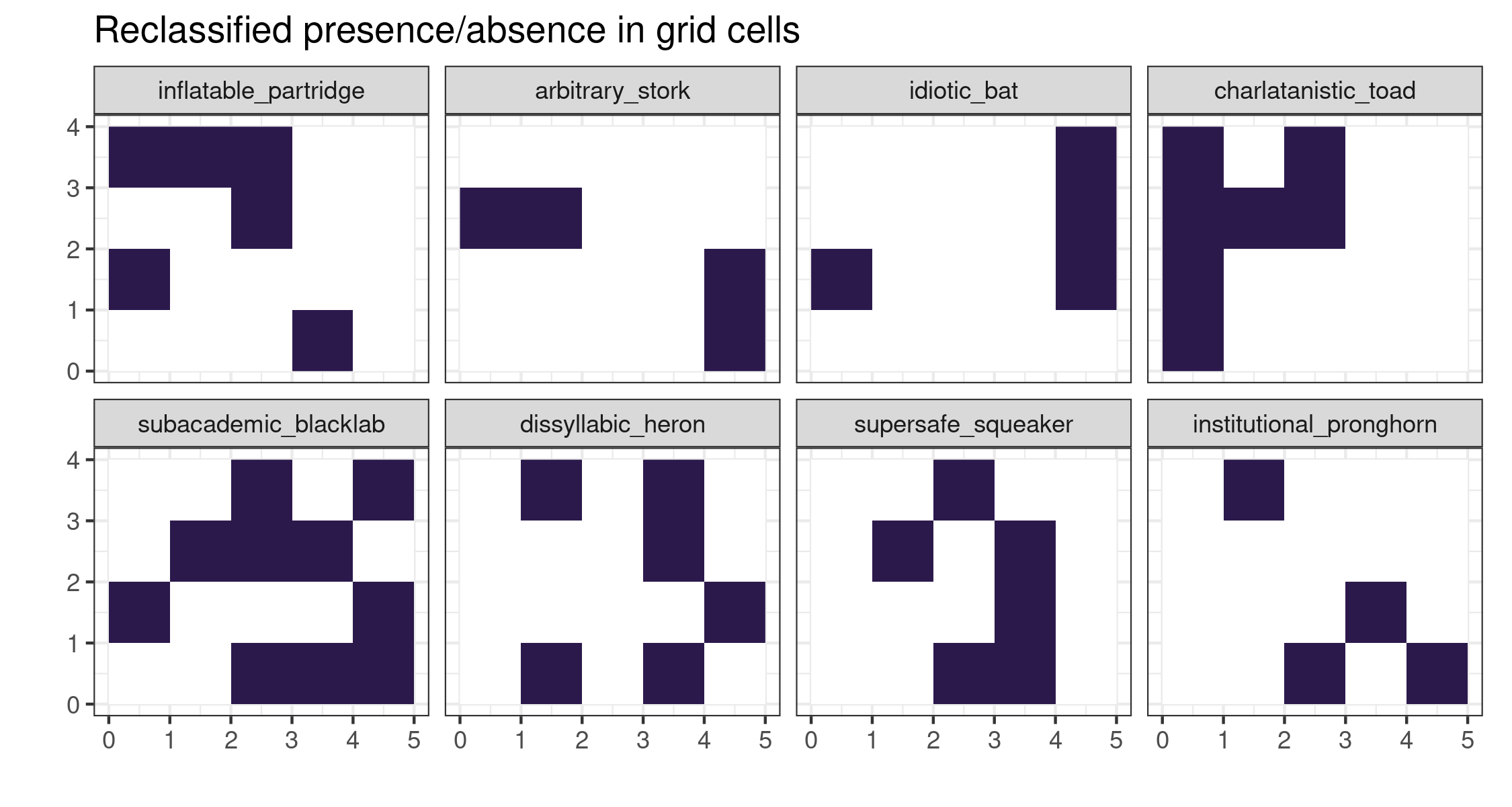
To sum these array dimensions, we use st_apply for the raster calculation. We apply sum to the dimensions with the xy coordinates to get the total value for each pixel.
# sum the array dimensions
cllspRich <-
  allspRC %>%
  st_apply(c("x", "y"), sum, na.rm = TRUE) %>%
  mutate(richness = if_else(sum == 0, NA_real_, sum)) %>%
  select(richness)
This is our richness raster, which we can plot now. The math checks out (i.e. the pixel values in this layer are the sum of all the 0/1 arrays)
# plot richness array
ggplot() +
  geom_stars(data = cllspRich) +
  coord_equal() +
  scale_fill_scico(palette = "davos", direction = -1, name = "Species Richness") +
  theme_bw() +
  labs(x = "", y = "")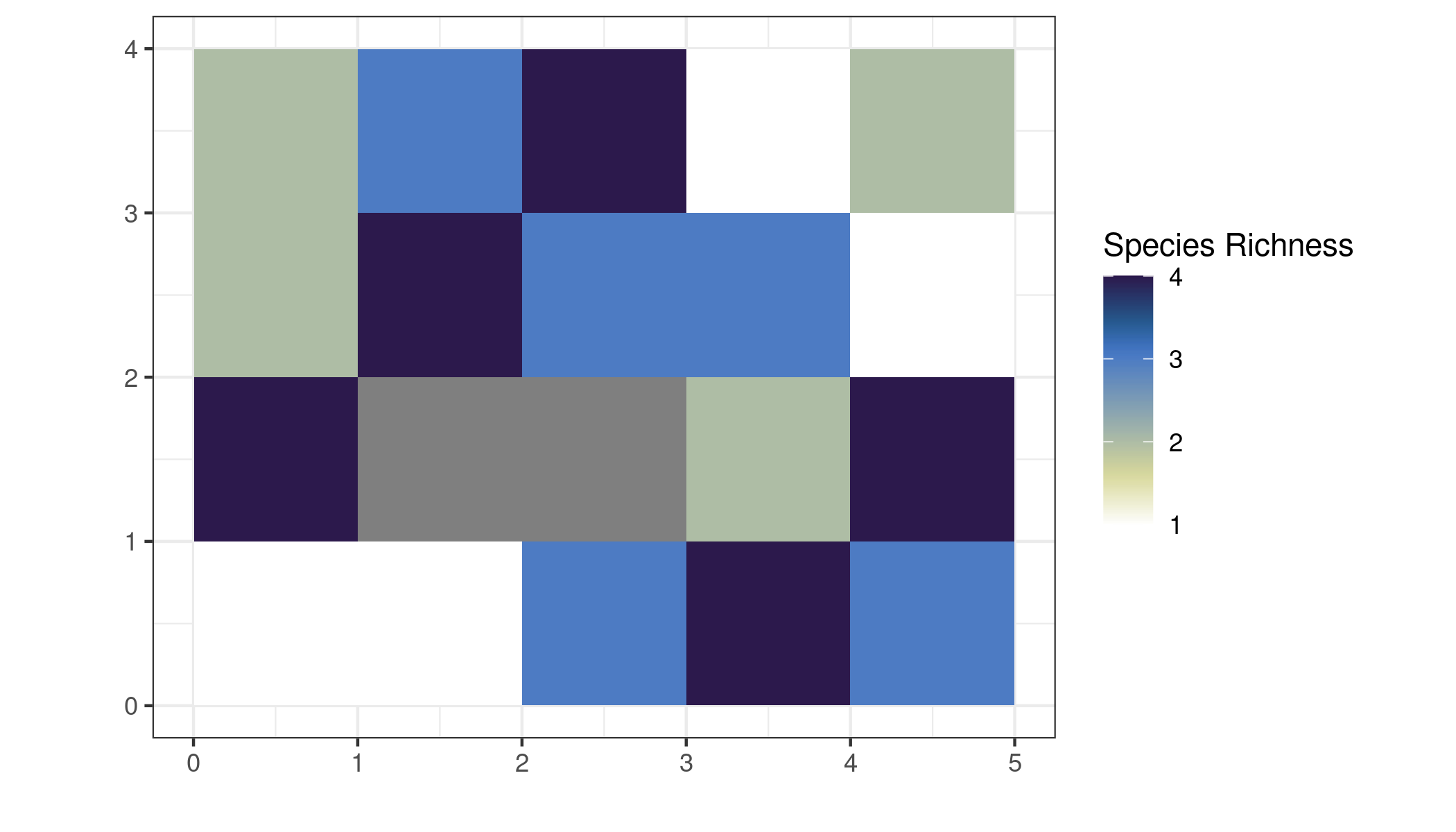
We can plot the stacks in “3d” with this approach by soil scientist Lauren O’Brien. After converting the rasters (stars) to polygons (simple features) and reshaping them, we can warp the geometries directly with dplyr::mutate.
# shearing
# to sf
allspmgsf <- allspsmg %>%
  split() %>%
  st_as_sf()
sppolys <- allspmgsf %>% gather("sp", "val", -geometry)
allspRCsf <- allspRC %>%
  split() %>%
  st_as_sf()
RCsppolys <- allspRCsf %>% gather("sp", "presence", -geometry)

# shear matric
sm <- matrix(c(2, 1.2, 0, 1), 2, 2)

# warp the polygon geometries
sppolys_tilt <- sppolys %>% mutate(geometry = geometry * sm)
RCsppolys_tilt <- RCsppolys %>% mutate(geometry = geometry * sm)
We can use patchwork to plot the original and reclassified stacks side by side
# 3d plot
sppolys_tilt %>%
  ggplot() +
  geom_sf(aes(fill = val)) +
  facet_wrap(~sp, ncol = 1) +
  scale_fill_scico(
    palette = "davos", direction = -1, name = "Habitat suitability",
    guide = guide_colorbar(title.position = "top", label.position = "bottom")
  ) +
  theme_void() +
  theme(legend.position = "bottom") +
  RCsppolys_tilt %>%
  ggplot() +
  geom_sf(aes(fill = presence)) +
  facet_wrap(~sp, ncol = 1) +
  scale_fill_scico(
    palette = "davos", direction = -1,
    breaks = c(0, 1), labels = c(0, 1),
    guide = guide_legend(
      title = "presence/absence",
      direction = "horizontal",
      title.position = "top",
      label.position = "bottom",
      label.hjust = 0.5,
      label.vjust = 1
    )
  ) +
  theme_void() +
  theme(legend.position = "bottom")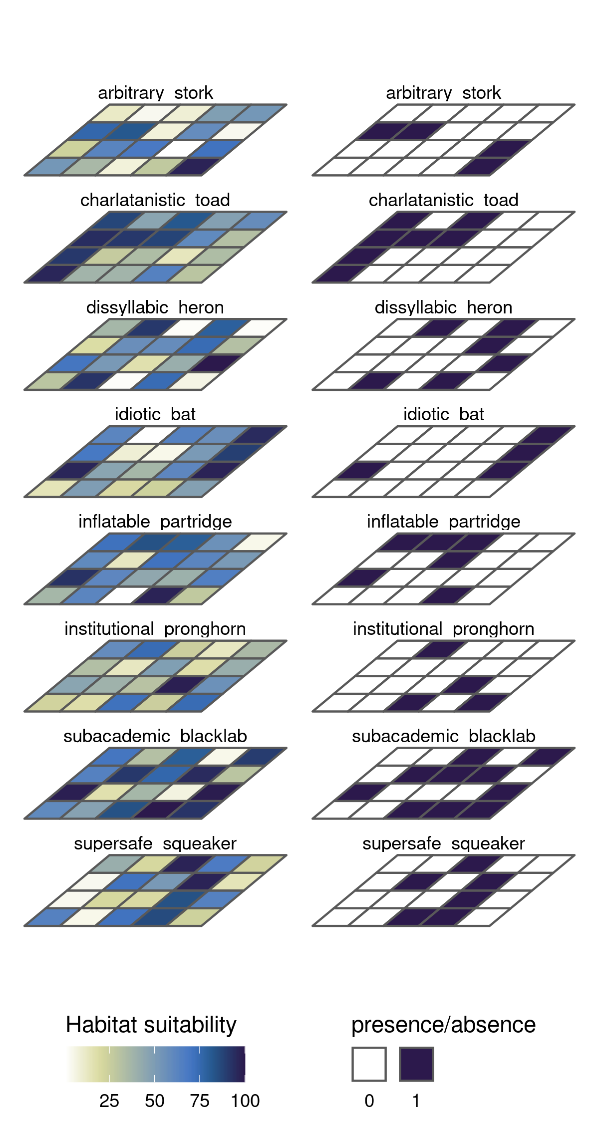
Working with real MaxEnt files
Let’s repeat the process with real raster files produced by MaxEnt. This example uses models of habitat suitability for 96 species of passerine birds in North America during the breeding season, produced by Diana Stralberg and archived on Zenodo.
The base map for our study area comes from rnaturalearth.
# base map
divpol <- rnaturalearth::ne_download(scale = "large", type = "countries", returnclass = "sf")
# reproject
divpolLamb <- st_transform(divpol, "+proj=lcc +lat_1=49 +lat_2=77 +lat_0=0 +lon_0=-95 +x_0=0 +y_0=0 +ellps=GRS80 +units=m +no_defs")
# subset north america
northam <- divpolLamb %>%
  filter(stringr::str_detect(SOVEREIGNT, "Canada|United States of America")) %>%
  filter(SUBREGION == "Northern America") %>%
  select(SOVEREIGNT)
I used fs and purrr to read all the asci raster files in a folder on my computer. The process for stacking them is the same as before.
# models, from Stralberg 2012 https://doi.org/10.5281/zenodo.3847272
brbirds <- dir_ls("PATH ON YOUR OWN COMPUTER", regexp = "asc$")
# read each raster, project it, and stack them all
brlist <- map(brbirds, read_stars)
brlistna <- map(brlist, st_set_crs, "+proj=lcc +lat_1=49 +lat_2=77 +lat_0=0 +lon_0=-95 +x_0=0 +y_0=0 +ellps=GRS80 +units=m +no_defs") # Canada Lambert
breedingbirds <- reduce(brlistna, c) %>%
  merge() %>%
  st_set_dimensions(names = c("x", "y", "sp"))
Let’s set a bounding box for our study area and plot 8 of these rasters, selected at random. Note how we can use dplyr::slice to subset arrays from our stars object.
# define a bounding box for plotting
limsboreal <- st_bbox(st_buffer(st_as_sf(breedingbirds), 20000))
# subset 4 species at random and plot
birds_subset <- breedingbirds %>% slice(sp, sample(1:96, 8))
# plot subset of species models
ggplot(northam) +
  geom_sf(fill = "#353535", color = "transparent") +
  geom_stars(data = birds_subset) +
  geom_sf(data = northam, fill = "transparent", size = 0.2, color = "black") +
  scale_fill_colormap("Habitat Suitability", na.value = "transparent", colormap = colormaps$portland) +
  ggthemes::theme_hc() +
  labs(x = "", y = "") +
  theme(
    panel.background = element_rect(fill = "#577399"),
    panel.border = element_rect(colour = "black", fill = "transparent"),
    legend.position = "bottom",
    panel.grid = element_line(size = 0.08)
  ) +
  coord_sf(
    xlim = c(limsboreal["xmin"], limsboreal["xmax"]),
    ylim = c(limsboreal["ymin"], limsboreal["ymax"])
  ) +
  facet_wrap(~sp, nrow = 2)
To calculate a species richness layer from these data, repeat the process from before to reclassify and sum the pixel values for all the arrays. Here all the steps are piped together.
# reclassify and sum to get species richness
breeding_birds_rich <-
  breedingbirds %>%
  mutate(presence = case_when(
    X > 70 ~ 1,
    TRUE ~ 0
  )) %>%
  select(presence) %>%
  st_apply(c("x", "y"), sum, na.rm = TRUE) %>%
  mutate(richness = if_else(sum == 0, NA_real_, sum)) %>%
  select(richness)
Now we can plot a nice richness map, built from MaxEnt models. This code has lots of optional aesthetic tweaks.
# plot the species richness
ggplot(northam) +
  geom_sf(fill = "#353535", color = "transparent") +
  geom_stars(data = breeding_birds_rich) +
  geom_sf(data = northam, fill = "transparent", size = 0.2, color = "black") +
  scico::scale_fill_scico(
    na.value = "transparent", palette = "lajolla", name = "Species richness",
    breaks = pretty(1:30),
    guide = guide_legend(
      title.position = "top",
      direction = "horizontal", nrow = 1,
      title.theme = element_text(size = 8, face = "bold"),
      label.theme = element_text(face = "bold")
    )
  ) +
  ggthemes::theme_hc(base_family = "Lato") +
  labs(x = "", y = "") +
  theme(
    panel.background = element_rect(fill = "#577399"),
    panel.border = element_rect(colour = "black", fill = "transparent"),
    legend.position = c(0.24, 0.1),
    legend.background = with_shadow(element_rect(fill = "#EBEBFF"), sigma = 3),
    panel.grid = element_line(size = 0.08)
  ) +
  labs(caption = "Passerine bird species richness, n=96. Breeding season") +
  coord_sf(
    xlim = c(limsboreal["xmin"], limsboreal["xmax"]),
    ylim = c(limsboreal["ymin"], limsboreal["ymax"])
  )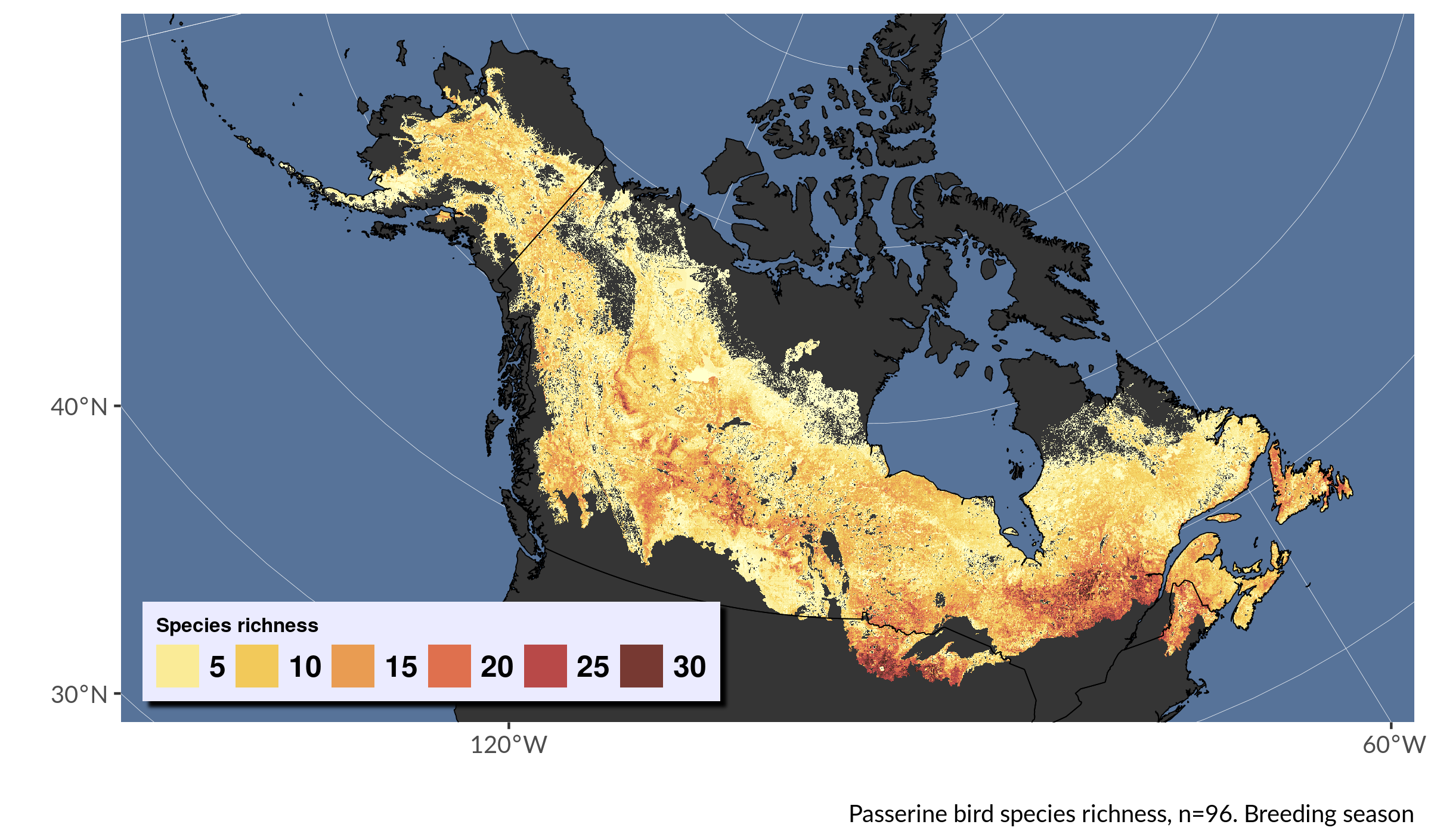
Looks pretty crisp.
That’s it. Contact me with any questions or if you get stuck. Have fun and stay safe!