Species richness analysis with R and sf

Este contenido está disponible en español aquí.

Updated Jan 2020. Fixed an error in the code that overestimated richness in empty cells, and added a case study.

Counting how many underlying features intersect a layer of interest is a very common geoprocessing task, and has always been possible with GIS software. I’ve been getting into the sf package to do spatial analyses in R, and wanted to document and share this approach for quantifying and plotting species richness.

The code below is a fully reproducible (as long as the relevant packages are installed). I chose Costa Rica as an example. First, we will generate random points iteratively, and a case study with bat species is at the end of the post. Shapefiles can be read easily into sf using st_read. Here, I calculated gridded richness for point data first and then for convex hulls because those are some of the most common approaches used nowadays.

These are the main steps in the process:

Setup

• subset a world map to get a single-country polygon
• generate a random number of random points within the country for n different ‘species’
• create smoothed convex hulls around each set of points

Geoprocessing

• generate a grid to cover our country polygon
• intersect and join the multipoint feature set and the convex hulls with the grid (separately). Note that we shouldn’t count the cells that don’t overlap the target feature.

Plotting

• plot the richness grids using perceptually-uniform and colorblind-friendly palettes using ggplot, scico and sf

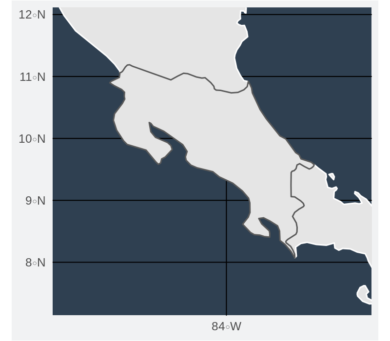
The different spatial elements look like this:

The blank map

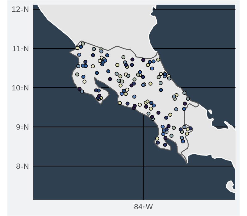
Randomly generated points for n ‘species’

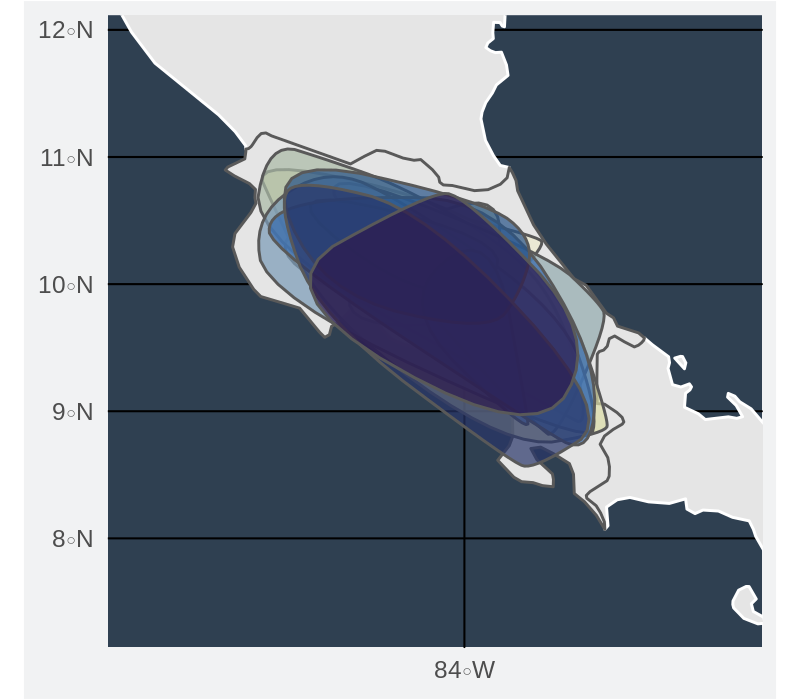
Smoothed convex hulls around the sets of points

Grid for calculating richness

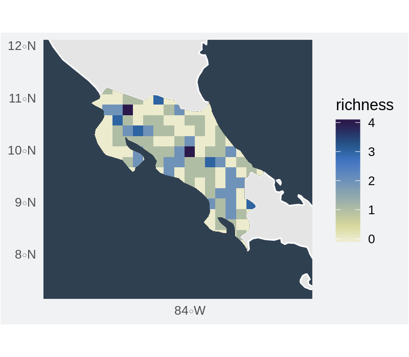
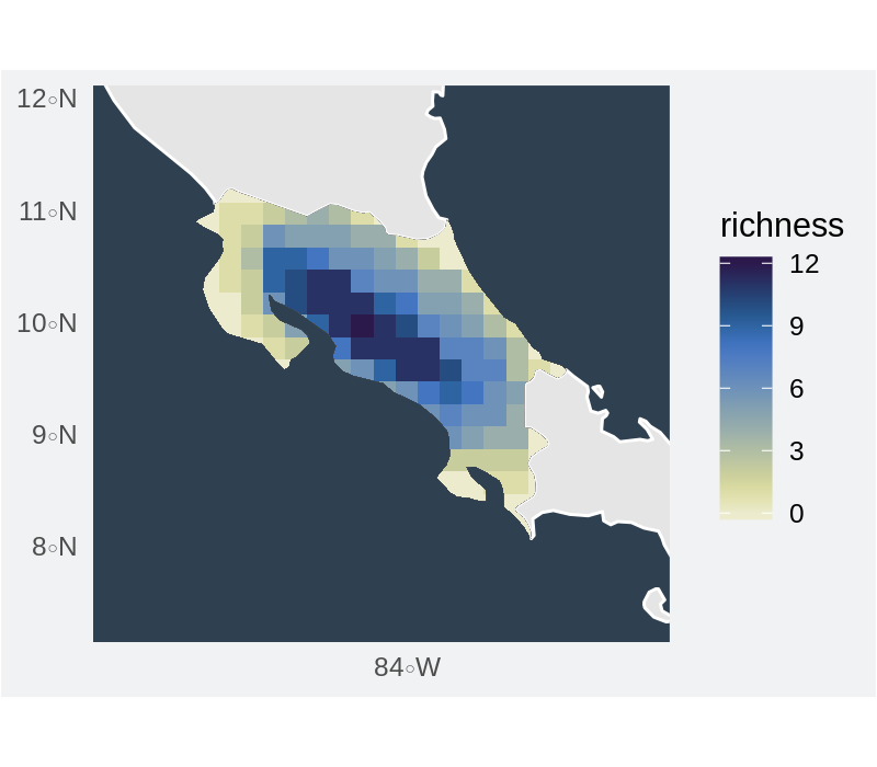
Gridded richness for points

Gridded richness for convex hulls

Notes:

The rerun function from purrr is awesome, I hadn’t seen it before but it is a very cool replacement for most basic for loops. I don’t know how I missed it.

When plotting, we use a bounding box and and the st_touches function with some tidyverse magic (slicing and plucking) to get the adjacent countries so we can add more context to our plot and focus in on our polygon of interest without having to set up the limits manually.

We counted the number of intersecting features using a grid, but this can also be done using political boundaries (states, municipalities, counties), vegetation types or any other layer of interest.

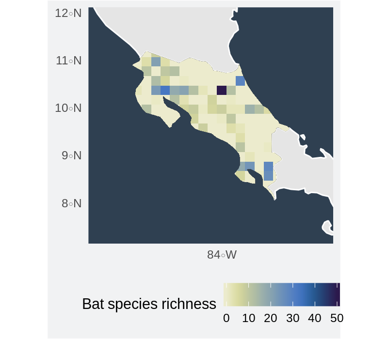
Case study

We can apply this same approach to real data, using point occurrence data (long/lat) in the form of an sf multipoint object. We’ll use some point data for bats, downloaded using rgbif. We can group and summarize the three-column table (species, longitude, and latitude) and assing the appropriate projection. The rest of the workflow is unchanged, and it can also be applied to shapefiles.

Bat species richness in Costa Rica

Any feedback is welcome.

R code:

# load packages
library(sf)
library(dplyr)
library(ggplot2)
library(scico)
library(rnaturalearth)
library(purrr)
library(smoothr)
library(rgbif)


# world map
worldMap <- ne_countries(scale = "medium", type = "countries", returnclass = "sf")

# country subset
CRpoly <- worldMap %>% filter(sovereignt == "Costa Rica")

# random points tables as a named list
sp_occ <- rerun(12, st_sample(CRpoly, sample(3:20, 1)))
names(sp_occ) <- paste0("sp_", letters[1:length(sp_occ)])

# to sf object
sflisss <-
  purrr::map(sp_occ, st_sf) %>%
  map2(., names(.), ~ mutate(.x, id = .y))

sp_occ_sf <- sflisss %>% reduce(rbind)

# to multipoint
sp_occ_sf <- sp_occ_sf %>%
  group_by(id) %>%
  summarise()

# trim to study area
limsCR <- st_buffer(CRpoly, dist = 0.7) %>% st_bbox()

# neighboring countries
adjacentPolys <- st_touches(CRpoly, worldMap)
neighbours <- worldMap %>% slice(pluck(adjacentPolys, 1))

# countries
divpolPlot <-
  ggplot() +
  geom_sf(data = neighbours, color = "white") +
  geom_sf(data = CRpoly) +
  coord_sf(
    xlim = c(limsCR["xmin"], limsCR["xmax"]),
    ylim = c(limsCR["ymin"], limsCR["ymax"])
  ) +
  scale_x_continuous(breaks = c(-84)) +
  theme(
    plot.background = element_rect(fill = "#f1f2f3"),
    panel.background = element_rect(fill = "#2F4051"),
    panel.grid = element_blank(),
    line = element_blank(),
    rect = element_blank()
  )
divpolPlot

# plot points
spPointsPlot <-
  ggplot() +
  geom_sf(data = neighbours, color = "white") +
  geom_sf(data = CRpoly) +
  geom_sf(data = sp_occ_sf, aes(fill = id), pch = 21) +
  scale_fill_scico_d(palette = "davos", direction = -1, end = 0.9, guide = FALSE) +
  coord_sf(
    xlim = c(limsCR["xmin"], limsCR["xmax"]),
    ylim = c(limsCR["ymin"], limsCR["ymax"])
  ) +
  scale_x_continuous(breaks = c(-84)) +
  theme(
    plot.background = element_rect(fill = "#f1f2f3"),
    panel.background = element_rect(fill = "#2F4051"),
    panel.grid = element_blank(),
    line = element_blank(),
    rect = element_blank()
  )
spPointsPlot

# convex hulls
spEOOs <- st_convex_hull(sp_occ_sf) %>% smooth()

# plot hulls
hullsPlot <-
  ggplot() +
  geom_sf(data = neighbours, color = "white") +
  geom_sf(data = CRpoly) +
  geom_sf(data = spEOOs, aes(fill = id), alpha = 0.7) +
  scale_fill_scico_d(palette = "davos", direction = -1, end = 0.9, guide = FALSE) +
  coord_sf(
    xlim = c(limsCR["xmin"], limsCR["xmax"]),
    ylim = c(limsCR["ymin"], limsCR["ymax"])
  ) +
  scale_x_continuous(breaks = c(-84)) +
  theme(
    plot.background = element_rect(fill = "#f1f2f3"),
    panel.background = element_rect(fill = "#2F4051"),
    panel.grid = element_blank(),
    line = element_blank(),
    rect = element_blank()
  )
hullsPlot


# grid
CRGrid <- CRpoly %>%
  st_make_grid(cellsize = 0.2) %>%
  st_intersection(CRpoly) %>%
  st_cast("MULTIPOLYGON") %>%
  st_sf() %>%
  mutate(cellid = row_number())

# cell richness
richness_grid <- CRGrid %>%
  st_join(sp_occ_sf) %>%
  mutate(overlap = ifelse(!is.na(id), 1, 0)) %>%
  group_by(cellid) %>%
  summarize(num_species = sum(overlap))

# richness for convex hulls
richness_gridEOO <- CRGrid %>%
  st_join(spEOOs) %>%
  mutate(overlap = ifelse(!is.na(id), 1, 0)) %>%
  group_by(cellid) %>%
  summarize(num_species = sum(overlap))

# empty grid
gridPlot <-
  ggplot() +
  geom_sf(data = neighbours, color = "white") +
  geom_sf(data = CRpoly) +
  geom_sf(data = CRGrid) +
  coord_sf(
    xlim = c(limsCR["xmin"], limsCR["xmax"]),
    ylim = c(limsCR["ymin"], limsCR["ymax"])
  ) +
  scale_x_continuous(breaks = c(-84)) +
  theme(
    plot.background = element_rect(fill = "#f1f2f3"),
    panel.background = element_rect(fill = "#2F4051"),
    panel.grid = element_blank(),
    line = element_blank(),
    rect = element_blank()
  )
gridPlot

# richness
gridRichCR <-
  ggplot(richness_grid) +
  geom_sf(data = neighbours, color = "white") +
  geom_sf(data = CRpoly, fill = "grey", size = 0.1) +
  geom_sf(aes(fill = num_species), color = NA) +
  scale_fill_scico(palette = "davos", direction = -1, end = 0.9) +
  coord_sf(
    xlim = c(limsCR["xmin"], limsCR["xmax"]),
    ylim = c(limsCR["ymin"], limsCR["ymax"])
  ) +
  scale_x_continuous(breaks = c(-84)) +
  theme(
    plot.background = element_rect(fill = "#f1f2f3"),
    panel.background = element_rect(fill = "#2F4051"),
    panel.grid = element_blank(),
    line = element_blank(),
    rect = element_blank()
  ) + labs(fill = "richness")
gridRichCR

# richness for convex hulls
gridRichCR_eoo <-
  ggplot(richness_gridEOO) +
  geom_sf(data = neighbours, color = "white") +
  geom_sf(data = CRpoly, fill = "grey", size = 0.1) +
  geom_sf(aes(fill = num_species), color = NA) +
  scale_fill_scico(palette = "davos", direction = -1, end = 0.9) +
  coord_sf(
    xlim = c(limsCR["xmin"], limsCR["xmax"]),
    ylim = c(limsCR["ymin"], limsCR["ymax"])
  ) +
  scale_x_continuous(breaks = c(-84)) +
  theme(
    plot.background = element_rect(fill = "#f1f2f3"),
    panel.background = element_rect(fill = "#2F4051"),
    panel.grid = element_blank(),
    line = element_blank(),
    rect = element_blank()
  ) + labs(fill = "richness")
gridRichCR_eoo

###################################################
# bat data
name_suggest(q = "chiroptera")
CRbatsout <- occ_search(
  orderKey = 734, country = "CR",
  basisOfRecord = "PRESERVED_SPECIMEN", limit = 3000
)$data
# species and lat long data
CRbatsXY <- CRbatsout %>%
  select(species, decimalLongitude, decimalLatitude) %>%
  na.omit()
# to sf object, specifying variables with coordinates and projection
CRbatsXYsf <- st_as_sf(CRbatsXY, coords = c("decimalLongitude", "decimalLatitude"), crs = 4326) %>%
  group_by(species) %>%
  summarize()

# plot points
batPointsPlot <-
  ggplot() +
  geom_sf(data = neighbours, color = "white") +
  geom_sf(data = CRpoly) +
  geom_sf(data = CRbatsXYsf, pch = 21) +
  coord_sf(
    xlim = c(limsCR["xmin"], limsCR["xmax"]),
    ylim = c(limsCR["ymin"], limsCR["ymax"])
  ) +
  scale_x_continuous(breaks = c(-84)) +
  theme(
    plot.background = element_rect(fill = "#f1f2f3"),
    panel.background = element_rect(fill = "#2F4051"),
    panel.grid = element_blank(),
    line = element_blank(),
    rect = element_blank()
  )
batPointsPlot

# bat richness
bat_richness_grid <- CRGrid %>%
  st_join(CRbatsXYsf) %>%
  mutate(overlap = ifelse(!is.na(species), 1, 0)) %>%
  group_by(cellid) %>%
  summarize(num_species = sum(overlap))

# plot
batRichCR <-
  ggplot(bat_richness_grid) +
  geom_sf(data = neighbours, color = "white") +
  geom_sf(data = CRpoly, fill = "grey", size = 0.1) +
  geom_sf(aes(fill = num_species), color = NA) +
  scale_fill_scico(palette = "davos", direction = -1, end = 0.9, name = "Bat species richness") +
  coord_sf(
    xlim = c(limsCR["xmin"], limsCR["xmax"]),
    ylim = c(limsCR["ymin"], limsCR["ymax"])
  ) +
  scale_x_continuous(breaks = c(-84)) +
  theme(
    plot.background = element_rect(fill = "#f1f2f3"),
    panel.background = element_rect(fill = "#2F4051"),
    panel.grid = element_blank(),
    legend.position = "bottom",
    line = element_blank(),
    rect = element_blank()
  ) + labs(fill = "richness")
batRichCR