What’s in a name?

With Mammal March Madness happening this month, I’ve been seeing a lot of common names for mammalian species in my Twitter feed and this year in particular two of the divisions are based directly on common names: Adjective mammals (e.g. Spectacled bear, pouched rat, clouded leopard, etc. ) and Two Animals One Mammal (e.g. bearcat, tiger quoll, hog badger, etc.). I recently had to figure out how to do text analysis for another project (in which I counted the most frequently-used words in the titles of hundreds of papers), so I wondered if I could apply the same analysis code to the common names for mammals (turns out I could). This post has two parts: Part One is a straightforward text analysis of word frequency, and Part Two is a nifty approach to quantifying name lengths.

Part 1: What are the most frequent words in the common names of thousands of mammalian species?

I’m doing this post for common names in English because these made for the largest dataset. Personally, I rarely use common names and we don’t really have nearly as many in Spanish - although some of the ones we have are pretty cool (e.g. tlacuachín, chungungo, and viejo de monte).

For this post we’ll use the tidytext R package and a massive list of common names for mammals that’s available thanks to the IUCN Red List assessments. All the code here should be fully reproducible, although you will probably need to install various packages first.

# load libraries
library(dplyr)
library(tidytext)
library(ggplot2)
library(forcats)
library(hrbrthemes)
library(ggalt)
library(extrafont)

## IUCN Red List data (download and tidy-up)
IUCN <- read.csv("https://raw.githubusercontent.com/ManuelaGonzalez/Who-is-Who/master/Mammals_2017_01_05.csv", stringsAsFactors=FALSE,strip.white=TRUE)
commNamesTax <- IUCN %>% select(Order,common_name=Common.names..Eng.,Genus,Species) %>% mutate(scName=paste(Genus,Species,sep=" "))

Once we download the IUCN data that we had from another post we use unnest_tokens() to split up the common names and end up with a row for every token (in this case words). With the words in this long format, we can easily quantify them using count(). Pretty cool and pretty simple.

## for all species
# saves entire title in `title_all` column
# splits up title column creating the `word` column -
# with a row for every token (word)

namesAll <- commNamesTax %>% mutate(names_all = common_name) %>% unnest_tokens(word, common_name)

# no need to remove stop words here
# quantify
by_wordAll <- namesAll %>% count(word, sort = TRUE)

I chose an arbitrary number of 20 top words to plot, using ggalt and hrbrthemes to make crisp and minimalist lollipop charts.

# prepare for plotting
loadfonts(device="win")

# plot
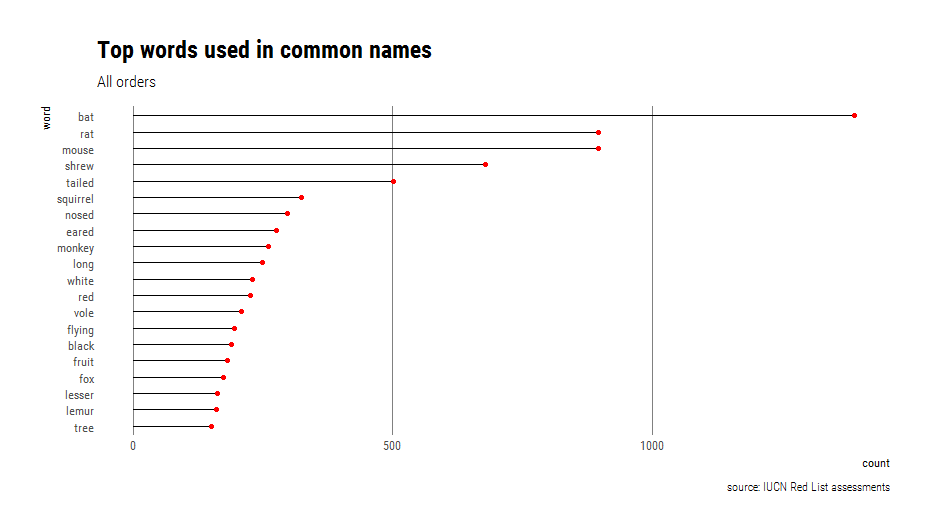
by_wordAll %>%
  top_n(20) %>% 
  ggplot(aes(x = fct_reorder(word, n), y = n)) +
  geom_lollipop(point.colour = "red",horizontal = F) +
  coord_flip() + 
  labs(title = 'Top words used in common names',
       subtitle="All orders", 
       caption="source: IUCN Red List assessments", x="word",y="count") +
  theme_ipsum_rc(grid="X")

Unsurprisingly, the top words for all orders reflect the names of the most diverse groups (rodents, bats, shrews and primates)

click to enlarge

To gain more insight, we can join the list of top words with the Parts of speech data frame that comes with tidytext. This dataset contains hundreds of thousands of English words from the Moby Project by Grady Ward, with each one tagged as “Noun”, “Adverb”, “Adjective”, or “Verb”, among other options. For some of the top terms there were multiple matches (for example: “flying” as an adjective, a noun, and a verb) but we can keep the first match using slice(). I also fixed up missing or mismatched terms manually using case_when().

I wrote a function to get the top n words, mainly as a way to document how non-standard evaluation works for unnest_tokens_ because I couldn’t find anything in the help files. Hint: it takes the arguments as character vectors.

# function to get top n
get_top_n_words <- function(x,y,n){
  allwords <- x %>% unnest_tokens_(c("word"),c(y))
  wordcount <- allwords %>% count(word,sort=TRUE)
  topwords <- wordcount %>% top_n(n)
  return(topwords)
}
# get top 20 words and tag them 
topWspeech <- get_top_n_words(commNamesTax,"common_name",20) %>% left_join(parts_of_speech)
# slice because of multiple matches
twspeechSliced <- topWspeech %>% group_by(word) %>% slice(1)
# fix missing or mismatched words manually
twspeechSliced <- twspeechSliced %>% ungroup %>% mutate(wordType= case_when(
  .$word=="tailed"~"Adjective",
  .$word=="nosed"~"Adjective",
  TRUE~ .$pos))

twspeechSliced %>% count(wordType) %>% mutate(wtypePercent= round(nn / sum(nn),2))

Among the top 20 words and ordered by frequency:

• Nouns outnumbered adjectives (55 vs 45%).
• Tails, noses, and ears are the most common features used to describe species.
• White, red, and black are the most common colors used to describe species.
• Long, flying, and lesser are the most common descriptors of different attributes or animals.

Even when expanding to the top 50 words, people’s last names did not make it into the list and the only place name is “African” at number 41. I kept looking and “Thomas’s” appears in a 10-way tie at number 125, with 33 species that include “Thomas’s” in their common name (e.g. Thomas’s Shrew Tenrec Microgale thomasi and Thomas’s Giant Deer Mouse Megadontomys thomasi). This is mainly because so many species have been named in dedication to British zoologist Oldfield Thomas.

We can then use faceting to repeat the plot for the six most speciose orders (>150 species) but with way less top words (for visibility).

# to redo by order
# work only with speciose orders (more than 150 species)
# group and subset the data
commNames_speciose <- commNamesTax %>% group_by(Order) %>%  filter(n() >= 150) 

# get top three words
topWbyOrder <- get_top_n_words(commNames_speciose,"common_name",3)

# plot with facetting
ggplot(topWbyOrder,aes(x = fct_reorder(word, n), y = n)) +
  geom_lollipop(point.colour = "red",horizontal = F) +
  coord_flip() + 
  labs(title = 'Top words used in common names',
       subtitle="by order", 
       caption="source: IUCN Red List assessments", x="word",y="count") +
  theme_ipsum_rc(grid="X")+
  facet_wrap(~Order)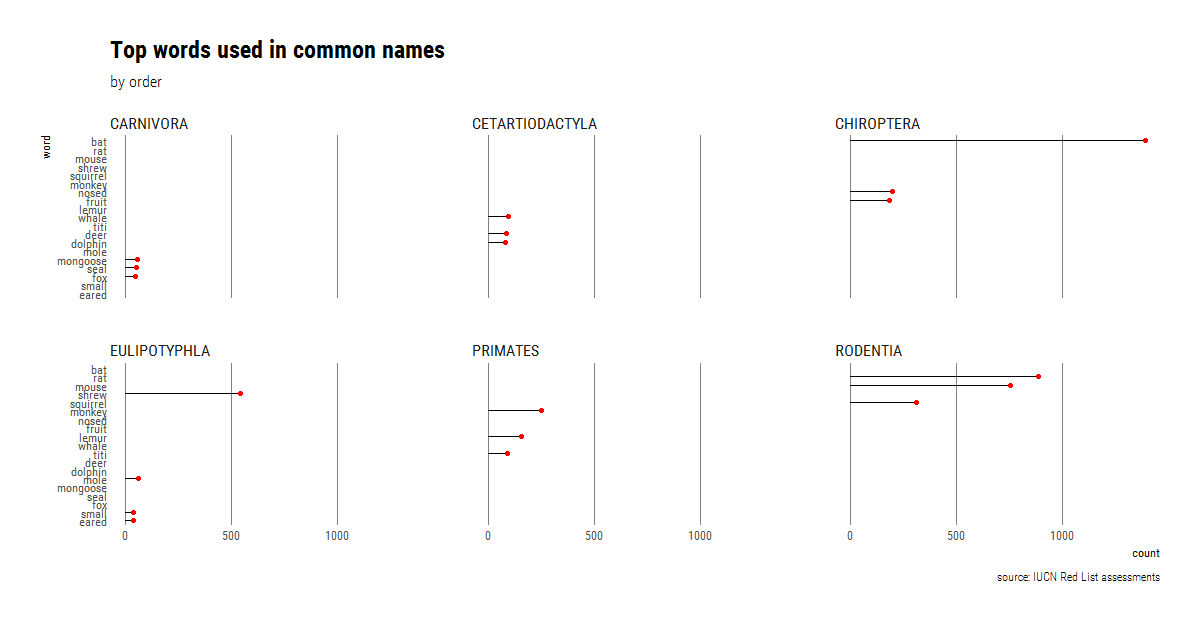

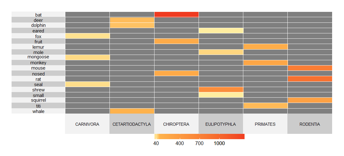
click to enlarge

We see that there is essentially no overlap in the most frequent words, but this is probably not the best way to visualize the high amount of mismatch. Instead, we can condense way more information using a heatmap, in this case created using Rebecca Barter’s superheat package. To make the heatmap, we take advantage of dplyr’s grouping capabilities before running the function to get the top n words. Afterwards all we need to do is change the data from long to wide format (using tidyr::spread in the same way we would have used reshape2::cast), and wrangle the row names into the order we want to use.

# change from long to wide format
library(tidyr)
topWbyOrderLong <- topWbyOrder %>% spread(Order,n)

# for heatmap
devtools::install_github("rlbarter/superheat")
library(superheat)

# wrangle row names
# this is because of the implicit sorting in tidyr
topWbyOrderLong <- as.data.frame(topWbyOrderLong)
topWbyOrderLong <- arrange(topWbyOrderLong,desc(word))
row.names(topWbyOrderLong) <- topWbyOrderLong$word
topWbyOrderLong$word <- NULL
# create heatmap
superheat(topWbyOrderLong,heat.col.scheme = "red",
          left.label.text.size = 4,
          bottom.label.text.size = 3.5,
          grid.hline.col = "white",
          grid.vline.col = "white")

The heatmap shows how there are no shared top words between the six most diverse orders, and also the frequency of each one.

click image to enlarge

Finally, I wrote a very crude function to generate new common names by just mashing up some of the popular words following three few simple formulas (adjective adjective noun, noun noun, adjective nounnoun).

# function to mash up common names
# inputs are: 
# dat: a datafame with a 'word' column 
## howmany: how many sets of common names to produce
newMammal <- function(dat,howmany){
  datSpeech <- dat %>% left_join(parts_of_speech) %>% 
    group_by(word) %>% slice(1) %>% 
    na.omit()
  adjs <- datSpeech %>% filter(pos=="Adjective")
  nouns <- datSpeech %>% filter(pos=="Noun")
  newMammA<- list()
  for (i in 1:howmany){
    newMammA[[i]] <- paste(sample(adjs$word,1,replace = F),sample(adjs$word,1,replace = F),sample(nouns$word,1,replace = F))
  }
  newMammB<- list()
  for (i in 1:howmany){
    newMammB[[i]] <- paste(sample(nouns$word,1,replace = F),sample(nouns$word,1,replace = F))
  }
  newMammC<- list()
  for (i in 1:howmany){
    newMammC[[i]] <- paste(sample(adjs$word,1,replace = F)," ",sample(nouns$word,1,replace = F),sample(nouns$word,1,replace = F),sep="")
  }
  newMamms <- c(newMammA,newMammB,newMammC)
  newMammsVecDF <- newMamms %>% simplify2array() %>% sample() %>% data.frame
  return(newMammsVecDF)
}

# try it out
newMammal(by_wordAll,10)

Most of the output makes no sense, but there were some funny ones, and I decided to draw a few with my epic MS Paint skills. Below is a sample of 100.

This function could be vastly improved by using more tags other than noun and adjective. For example, it’s possible to follow this post by Maëlle Salmon to separate animal names from other nouns.

100 random mashed up names

1 soricine dayakmar
2 pardine vampire
3 canarian lar
4 imposter dormouse
5 grizzled nepalese wisent
6 round birdlike graybeard
7  tumultuous hairless cochabamba
8  mesopotamian turkish capybara
9 bramble nyala
10 clara limestone
11 disk herring
12 sugar gazelle
13 margareta mashona
14 scaled basilanoubangui
15 siberian apevincent
16 sprightly unadorned bolo
17 cuban red ounce
18 hipped banded crescent
19 bidentate muleisland
20 wombat ringtail
21 toad niger
22 lipped herringnyala
23 limestone nonsense
24 himalayan gray saki
25  australasian tuftguadalcanal
26 riparian principal bobcat
27 lipped legged shadow
28 snouted zuluqueen
29 rough tubechipmunk
30 roan cottontailduiker
31 nimble black thomas
32 handed mountainkey
33 algerian colombian gold
34 rhino chad
35 naked equatorial podolsk
36 korean aurochsfur
37 thicket runner
38 prehensile bannershansi
39 gobi shark
40 colorful furred chiru
41 killer shadow
42 delectable mesquitelion
43 polynesian tamarmonk
44 colorado ethiopian bini
45 alexandrian shrewlike jones
46 caspian lorisvalais
47 rusty humpbacked humpback
48 dramatic sachathailand
49 larger ayecyrenaica
50 finless colorful langur
51 typical vietnammullah
52 squirrel jerboa
53 bush stick
54 woolly stony nord
55 wolf weasel
56 ibex markhor
57 pampas el
58  antarctic indochinese gervais
59  slaty proboscisdiadem
60  fur forest
61  mayan chacmasound
62  siam montague
63  swift destructive ebony
64  pallid baptistachannel
65  subalpine noble timor
66  river granada
67  micronesian rough runner
68  flores john
69  colored hispid st
70  pipistrelle heart
71  juan es
72  greenish caucasusochre
73  aardvark shan
74  serotine luciancascade
75  desperate finvole
76  skinned melanesian puku
77  trinidad pygmy
78  silent dainty santiago
79  thick quechuan cutch
80  sombre aloemagistrate
81  free santalowlands
82  zanzibar lynx
83  georgian tanzaniaanoa
84  eyra africa
85  baluchistan rock
86  lusitanian catgazelle
87  panamanian harmless fresno
88  marine angolaspot
89  cascade be
90  shaggy cyprian peccary
91  finless raneesound
92  swift kilimanjaropeak
93  serotine dianagoa
94  virginia ship
95  andaman amphibious mindoro
96  grand graceful straw
97  soda loyalty
98  mongolian swanlorenzo
99  bearing salim
100 wooly karoo kangaroo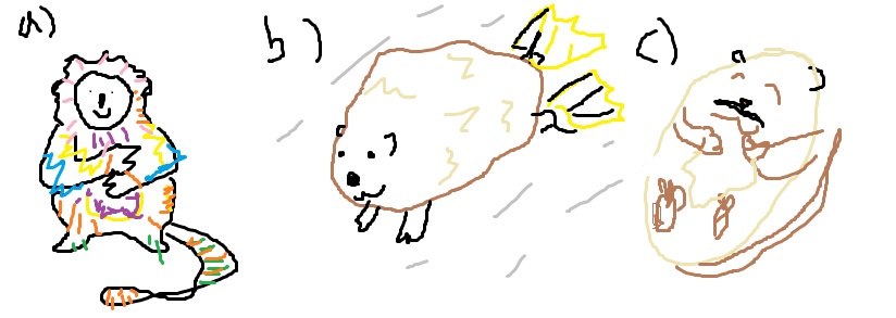

a) Finless colorful langur, b) Desperate finvole, c) Imposter dormouse

Part 2: Name lengths

Now we will quantify the length of different common names, in terms of both words and characters. Before doing that, it’s worth noting that of 5567 species in the dataset, 5350 have at least one common name listed. Also, 2407 species have >1 common names. The trick there was to use stringi’s stri_detect() to only keep rows that contain commas and then count the number of rows.

# part two: name lengths
library(stringi)
# how many sp have a common name
length(which(!is.na(commNamesTax$common_name)))

To count the number of names for species that have many, I kept it simple and used stringi to count the number of commas (plus one).

# count number of names
multNames <- commNamesTax %>% mutate(N_commonNames=(stri_count_fixed(common_name,",")+1))
# how many species have >1 common name ?
commNamesTax %>% filter(stri_detect_fixed(common_name,",")) %>% nrow()

Two species are tied with the highest number of common names (9): the grey wolf (aka. Timber Wolf, Arctic Wolf, Gray Wolf, Mexican Wolf, Plains Wolf, Common Wolf, Tundra Wolf, Wolf) and the wapiti (aka. Siberian Wapiti, McNeill’s Deer, Merriam’s Wapiti, Shou, Izubra/Manchurian Wapiti, Tien Shan Wapiti, Tule Elk, Alashan Wapiti).

Once we’ve counted the number of names, let’s check it out in histogram format.

# histogram
ggplot(multNames,aes(N_commonNames))+geom_histogram(binwidth = 1,fill="red",alpha=0.5)+
  theme_ipsum_rc(grid = "Y")+scale_x_continuous(breaks = c(1:9),label = c(1:9))+
  labs(title = 'Number of words in common names',
       subtitle="all orders", 
       caption="source: IUCN Red List assessments", x="number of names",y="count")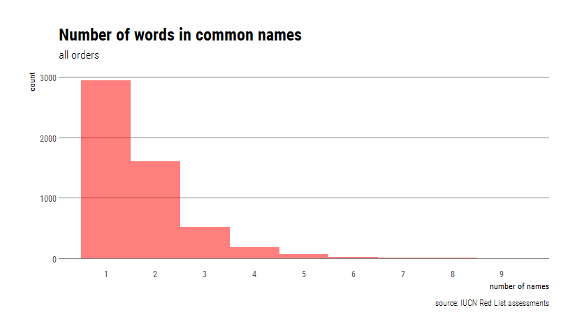

pretty skewed

To count the length of the common names in terms of characters, I had to make a choice about which name to keep for those species that had many. The simplest option was to keep the first one provided, using the separate() function in tidyr.

# separate using the commas
firstNames <- commNamesTax %>%  separate(common_name,",",into="FirstCname")
# count char lengths
firstNames$charlengths <- stri_length(firstNames$FirstCname)

The mammal with the shortest common name is the Kob (Kobus kob), an antelope found across sub-Saharan Africa. The species with the longest common name is the Black-crowned Central American Squirrel Monkey (Saimiri oerstedii), with a self-explanatory common name.

Now let’s look at the distribution of the number of characters, but using a density plot instead of a histogram.

# density plot
ggplot(firstNames,aes(charlengths))+geom_density(col="red")+
  theme_ipsum_rc(grid = "Y")+
  labs(title = 'Number of characters in common names',
       subtitle="all orders", 
       caption="source: IUCN Red List assessments", x="number of characters",y="density")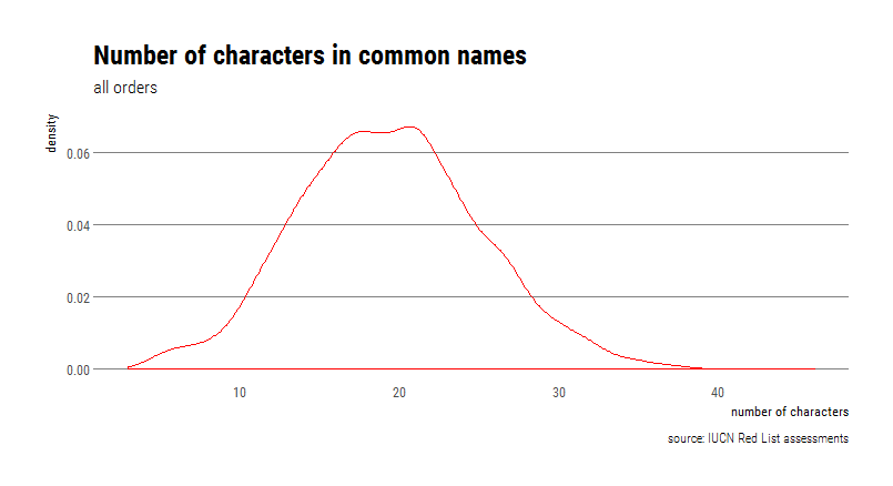

The distribution is much less skewed

That’s all, if you found this helpful please let me know, and also contact me if you find any mistakes in the code.

Go mammals!