If for some reason you haven’t seen the WeRateDogs twitter account (accurately described as ‘the best thing ever’ by barkpost.com), do that first then come back to this page.
For this entry I continue with my dog-themed posts, and I build on a few existing blog posts that analyzed tweets by We Rate Dogs. This post by David Montgomery examined how the dog ratings have changed over time, and this post by Bastian Greshake used TensorFlow to try and train an image classifier to rate the dogs. These two posts focus on the ratings, but I simply wanted to work with dog names.
I’ve written some posts on tweet/text analysis in the past, so to document my progress with string processing and text analysis I decided to build a corpus of dog names from those tweeted by We Rate Dogs. Also, some of the names are hilarious and I wanted to see them all together in a single list.
For this post, I did not download the tweets via an API, I worked with the csv file provided in David Montgomery’s post. I also used some of his code to extract the ratings for each dog. All the R code in the code blocks below should be reproducible, although you may need to install a few packages first.
Get the data and extract the ratings
# R script to analyze  tweets from @dog_rates.
# code in this block is modified from the script by David Montgomery, dhmontgomery.com. Released under the MIT License.

# Load libraries
library(dplyr)
library(stringi)
library(stringr)
library(rlist)
library(tidyr)

# read table from web
dogrates <- read.csv("https://raw.githubusercontent.com/dhmontgomery/personal-work/master/dogrates/dog_rates_tweets.csv", stringsAsFactors = F)
# duplicate the text col for later
dogrates$ogtext <- dogrates$text
## process the ratings
# Remove some extra characters
dogrates$text <- substr(dogrates$text, 3, nchar(dogrates$text)-1)
# Remove replies
dogrates <- filter(dogrates, substr(dogrates$text, 1, 1) != "@")
# Remove retweets
dogrates <- filter(dogrates, substr(dogrates$text, 1, 2) != "RT")
# Remove tweets without ratings out of 10
dogrates <- dogrates %>% filter(str_detect(text, "/10"))
# Split the text of each tweet along the character string "/10"
dogrates$rate <- str_split_fixed(dogrates$text, "/10", 2)
# Select just the first half of each tweet
dogrates$rate <- lapply(dogrates$rate, list.first)[1:1209]
# Remove some characters that sometimes precede the dog ratings, replacing them with spaces
dogrates$rate <- str_replace_all(dogrates$rate, "n"," ")
dogrates$rate <- str_replace_all(dogrates$rate, "[...]"," ")
dogrates$rate <- str_replace_all(dogrates$rate, "[(]"," ")
# Select the final word of each string — the numeric rating
dogrates$rate <- word(dogrates$rate, -1)
# Convert this final word from characters to numbers
dogrates$rate <- as.numeric(dogrates$rate)
# Hand-code one rating that didn't translate right
dogrates[292,5] <- 9.75
Processing strings to get a corpus of dog names
Once we used the data and code from the Pup Inflation blog post, we can use stringi and stringr and some regex to extract the names. Fortunately, the @dog_rates tweets have a pretty consistent format and use punctuation properly. From my experience following the account and from looking at the data frame, I identified three ways in which the dogs are introduced:
1.) This is X.
This is Aspen. She's never tasted a stick so succulent. On the verge of tears. A face of pure appreciation. 12/10 pic.twitter.com/VlyBzOXHEW
— WeRateDogs™ (@dog_rates) April 13, 2017
2.) Meet X.
Meet Odin. He's supposed to be giving directions but he'd rather look at u like that. Should probably buckle pup. 12/10 distracting as h*ck pic.twitter.com/1pSqUbLQ5Z
— WeRateDogs™ (@dog_rates) April 2, 2017
3.) Say hello to X.
Say hello to Alice. I'm told she enjoys car rides and smells good. 12/10 would give her everything she could ever want pic.twitter.com/yT4vw8y77x
— WeRateDogs™ (@dog_rates) April 17, 2017
Knowing this, we can use regular expressions to extract the text between each of those phrases and a period.
# use regex and stringi to extract names
dogrates$namesdogs <-str_extract_all(dogrates$text,c('(?<=hello to ).*?(?=\\.)|(?<=Meet ).*?(?=\\.)|(?<=This is ).*?(?=\\.)'),simplify=T)[,1]
Next, we remove empty rows and those that didn’t start with a capital letter. For example, the phrase “this is not a dog.” would be picked up by the regex but we don’t want it.
# filter to remove NA (blank) rows
dogratesFilt <- dogrates %>% filter(namesdogs!="")
# filter to remove rows that start with lowercase and don't typically have names
dogratesFilt <- dogratesFilt %>% filter(stri_detect_regex(namesdogs,"^[A-Z]"))
In some cases, the tweets include two dogs, so we use tidyr to unnest rows that contain two names (e.g. Sam and Max, Sam & Max) … I wish I knew about this function when I used to do all my unnesting by hand in Excel a few years ago.
# unnest rows with more than one name
dogRatesFiltUN <- dogratesFilt %>%
mutate(dnamessplit = strsplit(namesdogs, " and ")) %>%
unnest(dnamessplit)
# repeat with a different delimiter
dogRatesFiltUN <- dogRatesFiltUN %>% mutate(dnamessplit = strsplit(dnamessplit, " & ")) %>%
unnest(dnamessplit)Finally, we can sort out some special characters and clean up some rows manually.
# minor cleanup
dogRatesFiltUN$dnamessplit <- stri_replace_all_fixed(dogRatesFiltUN$dnamessplit,"his son ","")
dogRatesFiltUN$dnamessplit <- stri_replace_all_fixed(dogRatesFiltUN$dnamessplit,"her son ","")
dogRatesFiltUN$dnamessplit <- stri_replace_all_fixed(dogRatesFiltUN$dnamessplit,"her 2 pups ","")
# sort out special characters (unicode translations)
# see here http://www.utf8-chartable.de/unicode-utf8-table.pl?start=128&number=128&utf8=string-literal&unicodeinhtml=hex
dogRatesFiltUN$dnamessplit <- stri_replace_all_fixed(dogRatesFiltUN$dnamessplit,"\\xc3\\xa1","á")
dogRatesFiltUN$dnamessplit <- stri_replace_all_fixed(dogRatesFiltUN$dnamessplit,"\\xc3\\xa9","é")
dogRatesFiltUN$dnamessplit <- stri_replace_all_fixed(dogRatesFiltUN$dnamessplit,"\\xc3\\xb6","ö")
dogRatesFiltUN$dnamessplit <- stri_replace_all_fixed(dogRatesFiltUN$dnamessplit,"\\xc3\\xb3","ó")
At this point we have a table with 860 names, of which 634 are unique. We also have the ratings in a separate column thanks to David Montgomery’s code.
Here is a random sample of 50 names:
1                                   Toby
2                                 Spanky
3                                   Jeph
4                                Spencer
5                                 Oakley
6                                 Astrid
7                                Jeffrey
8                                Bentley
9                                 George
10                                 Lucia
11                                  Nida
12                              Finnegus
13             Devón (pronounced "Eric")
14                                 Kirby
15                                Brooks
16                                Brudge
17         Oliver (pronounced "Ricardo")
18                               Ralphie
19                                  Phil
20                                  Dave
21                                  Kyle
22                                 Scout
23                                    Bo
24                                  Bode
25                                Smokey
26                                   Jax
27                                 Lenox
28                                 Layla
29                                Oakley
30                                  Izzy
31                                Flávio
32 Enchilada (yes, that's her real name)
33                              Ashleigh
34             Logan, the Chow who lived
35                                   Leo
36                               Charlie
37                                 Tiger
38                                Pavlov
39                                  Link
40                                  Yoda
41                                  Berb
42                               Coleman
43                                 Misty
44                                  Taco
45                                Marley
46                                   Mia
47                                  Nala
48                                Ronnie
49                                 Craig
50                                  Lucy
To add a few more variables to play around with, we can use dplyr to summarize the data, getting the mean rating for each name. As a test, I also used the gender package to match the names with historical datasets (for people names) and add a vector of whether the name is for a male or female dog.
library(gender)
# assign genders to names based on historical data
# this is done in two steps because the gender function omits NAs
# get names and either m or f
matched <-  gender(dogRatesFiltUN$dnamessplit,years=c(2000,2012))
matched <- matched %>% select(dnamessplit=name,gender) %>% distinct()
# join with other tibble
dogRatesAll <- left_join(dogRatesFiltUN,matched)
# get the mean rate by name
dogRatesAll <- dogRatesAll %>% group_by(dnamessplit) %>% mutate(mRate=mean(rate),nmany=n()) %>% ungroup()
For visualization, I used ggplot to graph the 22 most common names in the corpus (ties are sorted in reverse alphabetical order) along with their sex and rating. I chose 22 arbitrarily, and even though the way I assigned male/female is questionable, we see that this list of 22 names is heavily biased towards names for male dogs. Keeping with the dog theme, I fed the ggplot object into the ggup function that I shared in my previous post. It can be sourced directly from a GH gist.
# plot the most common names
library(ggplot2)
library(ggalt)
library(forcats)
library(artyfarty)

# for specifying the axis text color
# filter, arrange, collect vector
gendervec <- dogRatesAll %>% select(nmany,dnamessplit,mRate,gender) %>% distinct() %>%
  top_n(22,nmany) %>% arrange(desc(nmany),desc(dnamessplit))%>% collect %>% .[["gender"]]
# replace with (randomly chosen) hex codes
gendercols <- case_when(gendervec=="male"~"#9502d1",
                        gendervec=="female"~"#176d10")

# ggplot object
dnames <- dogRatesAll %>% select(nmany,dnamessplit,mRate) %>% distinct() %>%
  top_n(22,nmany)%>%
  ggplot(aes(x=fct_reorder(dnamessplit,nmany),y=nmany,fill=mRate))+geom_bar(color="black",stat="identity")+
  coord_flip()+theme_bain()+scale_fill_gradient(low="white",high="#DAA520",name="rating")+
  theme(axis.text.y =  element_text(colour = rev(gendercols)))+
  labs(x="dog name",y="frequency")

# source the ggup function first
# (it requires lots of packages)
source("https://gist.githubusercontent.com/luisDVA/101374d9d6b569d887a1a2c7654cd3a4/raw/a98641561afbe7efa4d8ed6d7e1aac6f62abe2e2/ggpup.R")
ggpup(dnames)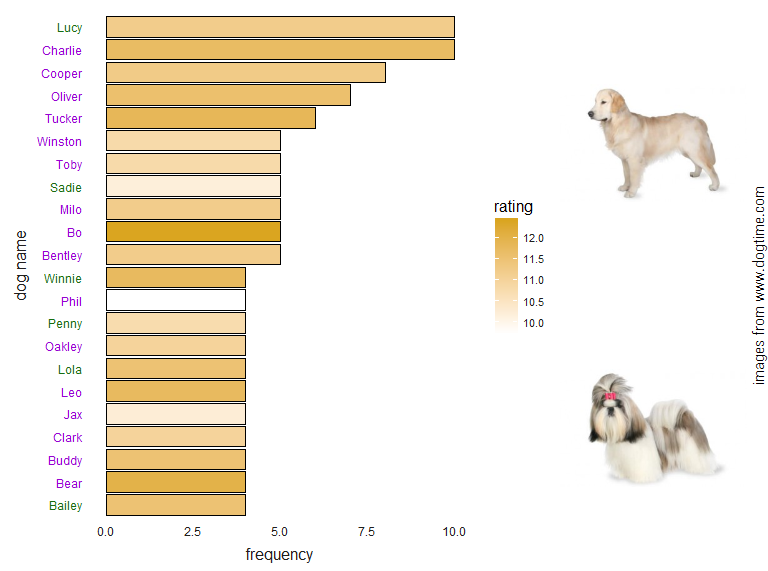
There were 507 names that only appear once, so I chose 22 of these at random to make a similar plot, but in this case the bars represent the rating instead of the frequency.
# repeat for names that only appear once (22 chosen at random)
randomDogs <- dogRatesAll %>% select(nmany,dnamessplit,mRate) %>% distinct() %>%
  filter(nmany==1) %>% sample_n(25)%>%
  ggplot(aes(x=fct_reorder(dnamessplit,mRate),y=mRate,fill=mRate))+geom_bar(color="black",stat="identity")+
  coord_flip()+theme_bain()+scale_fill_gradient(low="white",high="#DAA520",name="rating")+
  theme(axis.text.y =  element_text(colour = "black"))+
  labs(x="dog name",y="rating")

ggpup(randomDogs)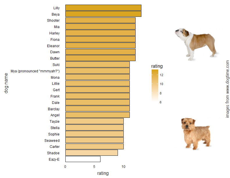
That’s all. Feel free to contact me if anything isn’t working or for any questions/comments.
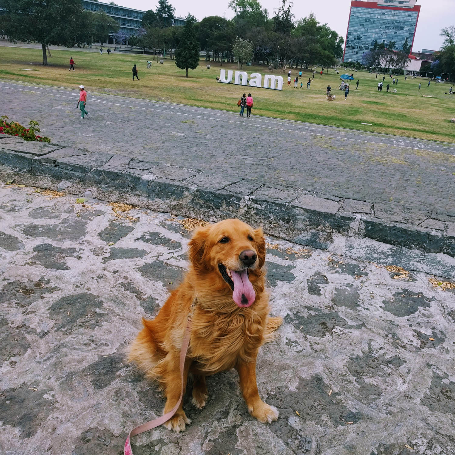
Side note: I checked and the name Luna only appears three times in this dataset, with a mean rating of 12.333. This is kind of a low rating, but that’s because I only submitted photos of my own Luna for rating recently. I assume she will probably get at least twice the maximum rating, approximately 30/10. Here she is.