
Update - June 2018 - an API is now necessary to download IUCN Red List data. This is easy to request though.
Red Lists of Threatened Species
This June, the European Red List of Birds revealed that almost 20% of bird species in Europe are facing extinction. This report is the result of three years of hard work by a consortium led by BirdLife International. This list, and similar recent publications (i.e the European Red List of marine fishes) are expected to guide conservation and policy work over the coming years. Assigning species into different threat categories can help to guide priorities for conservation investment, and produce different recommendations for conservation action for each category. Red Lists of threatened species can be compiled at various geographic levels (state/country/global), and they usually follow the rigurous quantitative methods set by the International Union for Conservation of Nature (IUCN). Red Lists are authoritative and objective systems for assessing large-scale, species-level extinction risk.
As we learn more about the threat status for more animal and plant groups through comprehensive Red List assessments, we can start identifying the biological factors and/or human pressures that explain why some species are more threatened than others. This usually involves using multivariate models to relate a species’ level of threat (e.g. Red List data) with information on its distribution, biology, and the threats it faces. These comparative analyses implement various statistical methods to overcome the fact that evolutionary relatedness can introduce apparent correlations between species’ traits.
Ordinal response
To date, most studies have treated Red List values of extinction risk as a continuous variable (i.e there are five main threat categories for living species, going from Least Concern -> Near Threatened -> Vulnerable -> Endangered -> Critically Endangered and they can be treated as a coarse continous index from 1 to 5). This approach assumes that the categories are continuously varying and evenly spaced. Instead, the Red List is an ordinal, categorical estimate of threat that represents an underlying continuous latent variable (the unknown true extinction risk). For example, the true difference in extinction risk may vary between categories of Least Concern and Near Threatened when compared with Critically Endangered and extinct.
The coarse continuous index approach can produce elevated type I error rates because it loses the variance structure of the original ordinal ranks. Problems arise when the ordinal ranks are separated by unequal distances along the underlying continuous variable that they measure, and we can’t know this beforehand. A growing number of papers have compared the results from ordinal vs continous models, and a simulation test by Matthews et al. (2011) found that the results can be consistent in most situations. The coarse continous approach isn’t necessarily wrong or misleading, but the sensitivity of models to different treatments of Red List response data is not always acknowledged.
Phylogenetic generalized linear mixed models
For my PhD research I studied extinction risk in mammals, and I used IUCN Red List data as the response variable. My co-supervisor and PCM guru Simon Blomberg convinced me to try and model the response as an ordinal index. At the time, only two studies had modeled Red List data as an ordered multinomial response, but both had potential non-indpendece issues. Liow et al. (2009) used nonphylogenetic proportional odds models; and González-Suárez & Revilla (2013) used taxonomically informed Generalised Linear Mixed Models. Initially, we tried to code ordinal logit models in JAGS - and while I struggled with the phylogenetic comparative aspect and the JAGS and Linux learning curves, a helpful Reddit user pointed me to the MCMCglmm package by Jarrod Hadfield.
MCMCglmm is an R package for fitting Generalised Linear Mixed Models using Markov chain Monte Carlo techniques. It draws on quantitative genetics methods, and I was very interested in how the it could incorporate phylogenetic information (as a covariance matrix representing the amount of shared evolutionary history between species), and use a probit link function to model ordinal responses. The package is widely-used and well-documented in mailing lists and discussion groups (and Jarrod was always helpful and patient whenever I pestered him on mailing lists or at conferences).
2013 paper
For my first thesis chapter, I investigated the relationship between extinction risk and quantitative properties of the mammalian phylogeny. I used MCMCglmm to fit Phylogenetic Generalised Linear Mixed Models (PGLMM; or the cooler-sounding Bayesian Phylogenetic Mixed Models, BPMM). This research was published in 2013 [OA link] and since then I’ve seen ordinal extinction risk modeling used to address some interesting questions for amphibians (De Lisle & Rowe 2015) and beetles (Seibold et al., 2015), using SAS and Mesquite routines that I haven’t looked into yet.
I’m still proud of having published the “first” ordinal/phylogenetic mammal extinction risk paper. I shared all my data and described the methods as thoroughly as I could, but I did not make my analysis and visualisation code available. On top of that I flaked when someone emailed me and requested the R code (sorry Jörg). I admit that at the time I was:
- Very sloppy at R and keeping track of scripts and data.
- Ashamed of my non-optimised code, annotated mostly in Spanish.
- Scared of blatant errors that I might have somehow missed, which would make the paper wrong and useless (despite supervisor review).
- Away on extended field work and conference travel.
I ended up perpetuating the annoying trend of not supplying materials “upon request” and I’d like to make it right. Below is a fully reproducible example for running and plotting a multivariate model of extinction risk in terrestrial carnivores (cliché/well-studied group) that takes into account phylogenetic relatedness between species, and the ordinal nature of Red List Data. It outlines what I did in the 2013 paper.
#rstats example code
This code is not very elegant, but it should be fully reproducible as long as you have an internet connection. Make sure you install the latest version of all the required packages and please let me know of any serious mistakes or cool data wrangling tips that I could incorporate.
Please contact me if you are interested in this sort of thing, or if you have any feedback.
Downloading and tidying trait data, phylogenetic tree and Red List status
# Load dplyr for data manipulation
require(dplyr)

# For reproducibility, read the table directly from the publication's URL
PantheriaWebAddress <- "http://esapubs.org/archive/ecol/e090/184/PanTHERIA_1-0_WR05_Aug2008.txt"
pantheria <- read.table(file=PantheriaWebAddress,header=TRUE,sep="\t",na.strings=c("-999","-999.00"),stringsAsFactors = FALSE)

# In this example we'll work with terrestrial carnivores
carnivora <- filter(pantheria,
                    MSW05_Order == "Carnivora"&
                    MSW05_Family!="Phocidae"&
                    MSW05_Family!="Otariidae"&
                    MSW05_Family!="Odobenidae")


# we'll use adult body mass (body size) and litter size for this exercise
# dplyr select can already be used to rename
carnivora <- select(carnivora,
                    Species = MSW05_Binomial,
                    BodySize = X5.1_AdultBodyMass_g,
                    LitterSize = X15.1_LitterSize)

# keep only complete cases
carnivora <- carnivora %>% filter(complete.cases(.))

# get the extinction risk values from the IUCN Red List API
# the letsR package can also query the Red List website but I've had http issues lately
require(taxize)
# get IUCN data summary
carnivoraIUCNSummary <- iucn_summary(carnivora$Species)
# extract threat status values
carnivoraIUCNdata <- iucn_status(carnivoraIUCNSummary)
# manipulate into dataframe of complete cases
carnivoraIUCNdata <- data.frame(carnivoraIUCNdata)
carnivoraIUCNdata$Species <- row.names(carnivoraIUCNdata)
carnivoraIUCNdata <- rename(carnivoraIUCNdata,Status = carnivoraIUCNdata)
carnivoraIUCNdata <- carnivoraIUCNdata %>% filter(complete.cases(.),Status!="DD")

# change Red List status to numerical index
require(letsR)
carnivoraIUCNdata$Status <- lets.iucncont(carnivoraIUCNdata$Status)+1

# merge tables
carnivoraFinal <- merge(carnivoraIUCNdata,carnivora,by="Species")
# logTransform body size
carnivoraFinal$lBodySize <- log(carnivoraFinal$BodySize)

# get a phylogeny
require(geiger)
# This resolved tree comes from Rolland et al (2014)
treeURL <- "http://journals.plos.org/plosbiology/article/asset?unique&id=info:doi/10.1371/journal.pbio.1001775.s001"
mammalPhylo <- read.tree(file=treeURL)

# trim tree to species in dataset
# but first, replace spaces to underscores to match tree tip formatting
carnivoraFinal$Species <- gsub(" ","_",carnivoraFinal$Species)
row.names(carnivoraFinal) <- carnivoraFinal$Species

# trim the phylogeny to match the data
carnPhylo <- treedata(mammalPhylo,carnivoraFinal)$phy

# drop the species not found in the tree
# treedata changes numeric to factor when dropping rows, so we drop them manually
toDrop <- setdiff(carnivoraFinal$Species,carnPhylo$tip.label)
carnivoraData <- carnivoraFinal[!rownames(carnivoraFinal) %in% toDrop, ]
For this example I’m ignoring known issues with missing data, taxonomy and synonyms, and phylogenetic uncertainty. All these issues can influence the model results and interpretation, and they should be addressed in a proper extinction risk study, especially one that aims to inform conservation.
- Missing data can be completed with thorough searches of recent or grey literature, or imputation techniques can fill in the gaps.
- Experience with the study group and open taxonomic resources can clear up the identity of species before running any analyses.
- Phylogenetic uncertainty can be addressed by performing MCMCglmm across multiple trees using the mulTree functions by Thomas Guillerme & Kevin Healy.
Running the model
# Now to run the multivariate model
require(MCMCglmm)

# create phylogenetic covariance matrix
Ainv <- inverseA(carnPhylo,nodes = "TIPS")$Ainv

# Define priors
# V prior follows suggested Gelman prior for ordinal regression by Gelman (2008), modified by J. Hadfield see function documentation
# R is fixed for an ordinal probit model. See function documentation
prior <- list (B=list(mu=rep(0,3), V=gelman.prior(~ lBodySize+LitterSize, data=carnivoraData, scale=1+pi^2/3)),
               R = list(V = 1, fix= 1),
               G = list(G1= list(V=1e-6, nu=-1)))

# run model

ERiskModel <- MCMCglmm(Status ~ lBodySize+LitterSize,
              data=carnivoraData, random=~Species,
              ginverse=list(Species=Ainv), family = "ordinal",
              prior= prior, nitt=600000, burnin=100000, thin=500)

# evaluate convergence
heidel.diag (ERiskModel$Sol) # Heidelberg and Welch (1983) diagnostic test
autocorr (ERiskModel$Sol) # autocorrelation of succesive samples (should be near 0)
plot (ERiskModel) # visual inspection of mixing properties of the MCMC chain

# explore results
summary (ERiskModel)
# summarize model for plotting
summModel <- summary(ERiskModel)
The number of iterations can be changed depending on hardware/patience. A few things I left out include: running parallel chains, and pooling chains with different starting values and then the corresponding convergence diagnostics. This particular model converged, and the model summary shows that the probabalities in the 95% credible region for the body size parameter estimate do not include zero (i.e. a “significant” positive relationship between body size and extinction risk).
| parameter | post.mean | l-95% CI | u-95% CI |
|---|---|---|---|
| (Intercept) | -3.19035 | -4.95698 | -1.67352 |
| body size | 0.37848 | 0.19934 | 0.54769 |
| litter size | -0.20584 | -0.40273 | 0.01897 |
No we can plot the effect of body size on extinction risk while the effects of litter size are kept constant. This works by calculating the probabilities of falling into each ordered category for any number of values of a linear predictor. The process is explained very well in this mailing list discussion and in the ordinal regression chapter of John Kruschke’s puppy-themed Bayesian Analysis book (see its accompanying blog entry). Originally I calculated these probabilities manually. Fortunately, Josh Wiley wrote the postMCMCglmm R package which contains functions to estimate predicted probabilites from an MCMCglmm object. In the end we have a dataframe of predicted probabilites (and CISs) for a range of body size values for each Red List category. Finally, I stacked the probabilities in a ggplot call using a color scheme that I think is pretty and effective (and technically colourblind and printer friendly).
Plotting the model results
# new data for prediction
# vectors for each predictor variable, based on the data

logBSize = seq(min(carnivoraData$lBodySize),max(carnivoraData$lBodySize), length.out=nrow(carnivoraData))
LitterSize = seq(min(carnivoraData$LitterSize),max(carnivoraData$LitterSize), length.out=nrow(carnivoraData))

# to plot the body size~threat relationship keeping the effect of litter size constant

newdat2 <- as.matrix(data.frame("(Intercept)"=1,
                      bodySize = logBSize,
                      LitterSize = median(LitterSize)))

# probabilities of falling into categories

require(devtools)
install_github ("postMCMCglmm", "JWiley")
require (postMCMCglmm)

## calculate predicted values

predCarn <- predict2(ERiskModel, X=newdat2, use = "all", Z=NULL, type = "response", varepsilon = 1)
summPredCarn <- summary (predCarn,level=0.99)

## combine predicted probs + HPD intervals with prediction data
predProbsCarn <- as.data.frame (cbind(do.call(rbind, rep(list(newdat2),5)), do.call(rbind,summPredCarn)))

## indicator for which level of the outcome
predProbsCarn$outcome <- factor (rep(c("LC","NT","VU","EN","CR"), each = nrow(summPredCarn[[1]])),
                                 levels=c("LC", "NT", "VU", "EN", "CR"))

# stack probabilities for the ordered categories

predProbsCarnLC <-  predProbsCarn %>%
  filter(outcome=="LC") %>%
  dplyr::select(M,LL,UL)%>%
  cbind(newdat2[,2])

predProbsCarnNT <-  predProbsCarn %>%
  filter(outcome=="NT") %>%
  dplyr::select(M,LL,UL)%>%
  mutate_each(funs(addProb = .+1)) %>%
  cbind(newdat2[,2])

predProbsCarnVU <-  predProbsCarn %>%
  filter(outcome=="VU") %>%
  dplyr::select(M,LL,UL)%>%
  mutate_each(funs(addProb = .+2)) %>%
  cbind(newdat2[,2])

predProbsCarnEN <-  predProbsCarn %>%
  filter(outcome=="EN") %>%
  dplyr::select(M,LL,UL)%>%
  mutate_each(funs(addProb = .+3)) %>%
  cbind(newdat2[,2])

predProbsCarnCR <-  predProbsCarn %>%
  filter(outcome=="EN") %>%
  dplyr::select(M,LL,UL)%>%
  mutate_each(funs(addProb = .+4)) %>%
  cbind(newdat2[,2])

predProbPlot <- rbind.data.frame(predProbsCarnLC,
                                 predProbsCarnNT,
                                 predProbsCarnVU,
                                 predProbsCarnEN,
                                 predProbsCarnCR)


predProbPlot <- rename(predProbPlot,bodySize=`newdat2[, 2]`)
predProbPlot$outcome <- factor (rep(c("LC","NT","VU","EN","CR"), each = nrow(summPredCarn[[1]])),
                                levels=c("LC", "NT", "VU", "EN", "CR"))

# plotting

require(ggplot2)

 ggplot (predProbPlot, aes(x = bodySize, y = M, colour = outcome)) +
  geom_ribbon(aes(ymin = LL, ymax = UL, fill = outcome), alpha = .25) +
  geom_line(size=2)+
  scale_y_continuous(breaks=seq(0.5,4.5,by=1),
                     labels=c("LC", "NT", "VU", "EN", "CR"),expand=c(0,0))+
  scale_x_continuous(expand=c(0,0))+
  ylab("threat category")+xlab("log(body size)")+
  scale_color_manual(values=c("#fed976","#feb24c","#fd8d3c","#f03b20","#bd0026"),name="Red List Status")+
  scale_fill_manual(values=c("#fed976","#feb24c","#fd8d3c","#f03b20","#bd0026"), guide=FALSE)+
  theme_classic()+theme(legend.position = "none",axis.ticks.y = element_blank())+
   geom_hline(yintercept=seq(0:4),by=1)
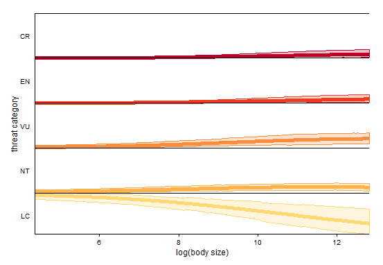
The probability of being at the Least Concern threat category is highest for smaller-bodied species, and it decreases with increasing body size. The interpretation for the other categories is done the same way.