
Hip hop and basketball have always had a unique and close relationship, so it is not surprising when player names and various terms from the sport appear in rap lyrics. This post works though the R code needed to find NBA player names in the lyrics of ~4000 songs from 20 hip hop artists and plotting the resulting patterns.
I’m writing this mainly to document several tricks and hacks for working with and ultimately plotting large(ish) volumes of text-based data. The choice of artists is a mix of rappers that I listen to, and others that seemed well-represented in the Genius lyrics data.
The overall workflow is split into getting a hold of lyrics and NBA player names and finding out: which artists are mentioning which players in their songs, and which players get mentioned most.
Getting the lyrics
Until last year, lyrics could be accessed from the Genius website (a massive collection of song lyrics and crowd-sourced annotations) via the Genius API with the geniusr package. At present, because of changes to the Genius API and legal terms, we can no longer fetch lyrics directly with geniusr directly without legally-gray webscraping (if you must, the relevant geniusr functions can be patched with the advice in this issue and they’ll work fine - but see here for more information).
This little example uses many cool packages, let’s set them up first.
# bball player names in hip hop
# Load libraries ----
library(geniusr)   # [github::ewenme/geniusr] v1.2.0.9000
library(nbastatR)  # [github::abresler/nbastatR] v0.1.1506
library(rvest)     # CRAN v1.0.2
library(xml2)      # CRAN v1.3.3
library(rlang)     # CRAN v1.0.1
library(tibble)    # CRAN v3.1.6
library(dplyr)     # CRAN v1.0.8
library(purrr)     # CRAN v0.3.4
library(stringr)   # CRAN v1.4.0
library(tidytext)  # CRAN v0.3.2
library(tidyr)     # CRAN v1.2.0
library(forcats)   # CRAN v0.5.1
library(ggplot2)   # CRAN v3.3.5
library(artyfarty) # [github::datarootsio/artyfarty] v0.0.1
library(ggfittext) # CRAN v0.9.1
library(ggtext)    # CRAN v0.1.1
library(scico)     # CRAN v1.3.0
library(extrafont) # CRAN v0.17
library(fuzzyjoin) # CRAN v0.1.6
Back when the API still produced tibbles with lyrics, I searched for the respective ID for the following artists, and used each artist ID to obtain a vector with all the unique song IDS for each of the following artists:
The artist names:
c("Migos", "Ghostface Killah", "2 Chainz", "G-Unit", "Beastie Boys", "Army of the Pharaohs", "Flatbush Zombies",
"R.A. The Rugged Man", "Das EFX", "Jedi Mind Tricks", "Gang Starr", "Mobb Deep", "Wu-Tang Clan", "Kool G Rap",
"DMX", "MF DOOM", "213", "Goodie Mob", "Sage Francis")
Here are examples for two of the artists. Each vector of song ids gets named consistently, so we can combine them all later (I didn’t iterate here so I could check that I was getting the correct matches for each search term).
search_artist("outerspace") # 1836
OSall <- geniusr::get_artist_songs_df(1836)
allOSsong_ids <- OSall %>% pull(song_id)

geniusr::search_artist("gang starr") # 220
GSTall <- geniusr::get_artist_songs_df(220)
allGSTsong_ids <- GSTall %>% pull(song_id)
Once we found all the artists we wanted, we can get the vector objects from our enviroment with mget.
### combine all artists
all_song_ids <- flatten_chr(mget(ls(pattern = "^all")))
To get all the lyrics, we can iterate over the final vector of song ID (with a multi-statement lambda function to add some time between requests and not spam the server).
# iterate and get all song lyrics
all_lyricsdf <- map_df(all_song_ids,~ {
  Sys.sleep(sample(seq(0.5,1,0.25),1))
  get_lyrics_id(song_id = .x)})
The resulting tibble has >200,000 rows, one per line for roughly 4000 songs. Here’s a random sample of 10 rows.
all_lyrsdf %>% slice_sample(n=10)# A tibble: 10 × 6
line section_name section_artist song_name artist_name song_id
<chr> <chr> <chr> <chr> <chr> <chr>
1 I know what it… Verse 3 Young Buck Footprin… G-Unit 20762
2 Dracos and MAC… Verse 3 Offset & Quavo Racks 2 … Migos 5555420
3 I don't trust … Hook Quavo Trust No… Migos 2340835
4 Leaving my dre… Verse 3 Offset White Sa… Migos 3468920
5 All you know i… Verse 3 2 Chainz I Said Me 2 Chainz 4346684
6 Pickin my mark… Havoc Mobb Deep It’s Over Mobb Deep 33514
7 You should see… Chorus The Notorious… The Dang… R.A. The R… 136500
8 Close your ear… Intro Havoc So Long Mobb Deep 33536
9 I'm off style … Verse 3 Ghostface Kil… Ron O’Ne… Wu-Tang Cl… 491657
10 A lousy condit… Yeeeaah, yo… Louis Logic Over the… Louis Logic 29385 For reference, this post by Tom MacNamara also shows how to get and visualize lyrics from the same data source.
Text analysis
For this exercise, let’s split up (tokenize) all the lines into bigrams (consecutive sequences of two words) with unnest_token from tidytext. For the next step, it’s also convenient to add new columns with the bigrams split into separate columns.
# tokenize
lyric_bigrams <- all_lyrsdf %>% unnest_tokens(BGlyric,line, token = "ngrams", n=2) %>%
  filter(!is.na(BGlyric)) %>% separate(BGlyric,into=c("w1","w2"),sep = " ",remove = FALSE)
To reduce the number of comparisons and because people’s names are the whole point of this exercise, we can filter out the rows in the lyrics data which match any of the words in a custom list of stop words (extremely common words not useful for analysis, such as “the”, “of”, “to”, etc.) from a generic text file.
# stopwords
stopWords <- tibble(word=readr::read_lines("minimal-stop.txt"))
lir <- lyric_bigrams %>% filter(!w1 %in% stopWords$word & !w2 %in% stopWords$word)
Player names
The dictionary_bref_players() function from nbastatR will get us a dictionary of NBA player names (from the Basketball Reference website) in tibble form. No arguments are needed, but we can just remove names from the BAA league to simplify the process.
# NBA player names
playerNames <- nbastatR::dictionary_bref_players()
playerNames <- playerNames %>% filter(!is.na(countSeasons))
Fuzzy joining
For a more flexible merge of the two columns (the player names and the lyric bigrams), the fuzzyjoin package implements various methods for fuzzy string matching, to allow for minor variations in spelling. For no particular reason, I matched the columns with Levenshtein distance and a maximum distance of one. Be aware that all these comparisons consume a lot of memory.
joineddfs <-
  stringdist_left_join(playerNames,
                       lir,by=c("namePlayerBREF"="BGlyric"),max_dist=1,
                       method=c("lv"),
                       ignore_case=TRUE)
After some cleaning and deduplicating, for the main visualization we can count how many times each player was mentioned. I manually filtered out eight homonyms (I doubt that lyrics mentioning Michael Jackson or Mel Gibson referred to a Knicks point guard (1987-1990) or a guard for the Lakers in 1964, respectively). I most likely missed some.
# clean and deduplicate
playermentions <- joineddfs %>% filter(!is.na(BGlyric)) %>%
  distinct(song_id,BGlyric,.keep_all = TRUE)
# remove homonyms
mentions_countF <-
  mentions_count %>% filter(!namePlayerBREF %in% c("Michael Jackson","Dan King",
                                                   "Bill Smith","Ed Horton","Larry Sanders",
                                                   "Bobby Brown","Mel Gibson","Harry Davis"))
The final data for plotting results from a series of hacks to rank and arrange the names according to their number of mentions (cur_group_id() is our friend here), and then to ‘conditionally’ wrap some of the names so they fit nicely in the plot. My improvised approach for categories with many names was to stack them side by side with lead, slice out every other row (note the %% operator), then put things back together.
# prepare data for plotting
freqsPL <-
  mentions_countF %>% add_count(n,name = "ncat") %>%
  mutate(nr=forcats::fct_inorder(as.factor(n))) %>%
  group_by(nr) %>%
  arrange(desc(namePlayerBREF),.by_group = TRUE) %>%
  mutate(rank = cur_group_id()) %>%
  mutate(forticks=paste0(n))

freqsPLtop <- freqsPL %>% filter(n>2) %>%
  mutate(namePlayerBREF=str_wrap(namePlayerBREF,width = 12))
freqsPLmid <- freqsPL %>% filter(n==2) %>%
  mutate(namePlayerBREF=paste(namePlayerBREF," ", lead(namePlayerBREF))) %>%
  slice(which(row_number() %% 2 == 1))
freqsPLbottom <- freqsPL %>% filter(n==1) %>%
  mutate(namePlayerBREF=paste(namePlayerBREF," ", lead(namePlayerBREF))) %>%
  slice(which(row_number() %% 2 == 1))

allfreqsPL <- bind_rows(freqsPLtop,freqsPLmid,freqsPLbottom) %>%
  mutate(namePlayerBREF=str_remove(namePlayerBREF," NA"))
Plotting
Before the plotting, lets set up a gradient background for the plot panel following this entry, and a separate tibble for a colorful annotation using ggtext.
  # gradient background grob
g <- grid::rasterGrob(c("#272822","black"), width=unit(1,"npc"), height = unit(1,"npc"),
                      interpolate = TRUE)
# custom text annotation
forsubtitle <-
  tibble(label = "<span style = 'color: #0F58FF;'>**3988**</span> songs from <span style = 'color: #0F58FF;'>**21**</span> artists <br> <span style = 'color: #F95C09;'>**5022**</span> player names",
         x = 0.7, y = 35)
The data now looks like this:
> allfreqsPL
# A tibble: 90 × 6
# Groups:   nr [8]
   namePlayerBREF          n  ncat nr     rank forticks
   <chr>               <int> <int> <fct> <int> <chr>
 1 "Michael\nJordan"       9     1 9         1 9
 2 "Scottie\nPippen"       8     1 8         2 8
 3 "Shaquille\nO'Neal"     6     3 6         3 6
 4 "Reggie\nMiller"        6     3 6         3 6
 5 "LeBron James"          6     3 6         3 6
 6 "Yao Ming"              5     6 5         4 5
 7 "Steve Nash"            5     6 5         4 5
 8 "Shawn Kemp"            5     6 5         4 5
 9 "Paul Pierce"           5     6 5         4 5
10 "Gilbert\nArenas"       5     6 5         4 5
# … with 80 more rows
Now we can plot the mentions as text stacked inside bars, using ggfittext for dynamic resizing. The ‘Rock Salt’ font is from Google Fonts, downloaded to my Linux system using Typecatcher and shown using extrafont.
ggplot(allfreqsPL,aes(x=factor(rank),y= n,label=namePlayerBREF))+
  annotation_custom(g, xmin=-Inf, xmax=Inf, ymin=-Inf, ymax=Inf) +
  geom_bar_text(position="stack",min.size = 2,
                family="Rock Salt",reflow = F,
                grow = TRUE, place="left",outside = TRUE)+
  scale_x_discrete(breaks=1:8,labels=unique(freqsPL$forticks),
                   expand = expansion(add=c(0.01,0.5)))+
  scale_y_continuous(expand = c(0.01,0.01))+
  geom_richtext(data=forsubtitle, aes(x=x,y=y,label=label),
                color="white",family="Lato Thin",size=9,
                fill = NA, label.color = NA,hjust= 0)+
  theme(panel.grid.major = element_blank(),
        axis.line.y = element_blank(),
        axis.text.y = element_blank(),
        axis.ticks.y = element_blank(),
        panel.background=element_blank(),
        panel.border = element_blank(),
        plot.background=element_rect(fill = "black"),
        plot.title = element_text(vjust = -0.5,size=32, hjust=0.03,
                                  family = "Lato Medium",color="white"),
        axis.text.x = element_text(family="Lato Heavy",size=19),
        axis.ticks = element_blank(),
        axis.title.x = element_text(color="white",size=17))+
  labs(x="mentions",y="",
       title="NBA players mentioned in hip hop songs")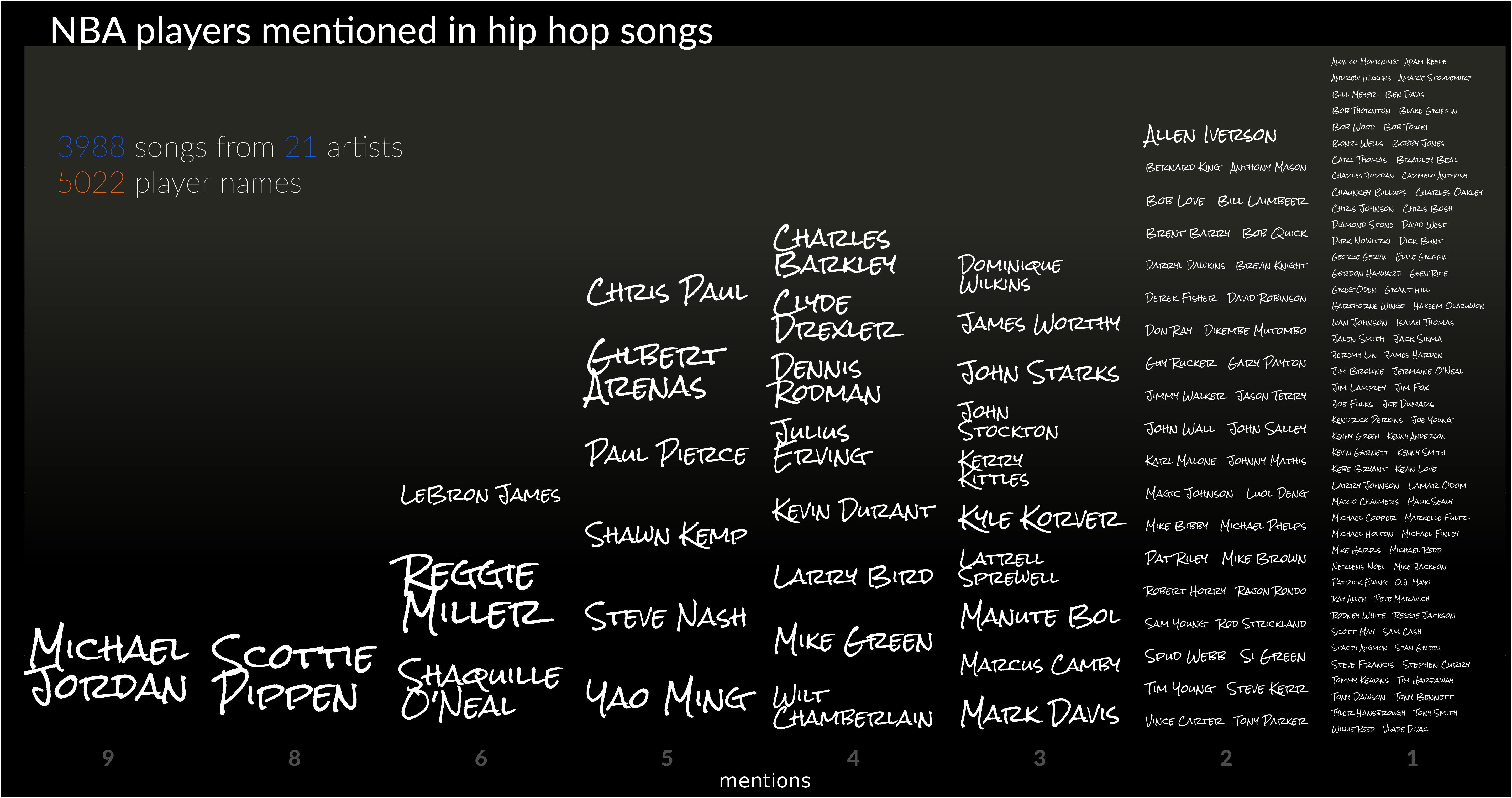
As a complement, we can figure out the number of distinct players mentioned by the different artists.
# to get player per artist
lyrsplyrs <-
  joineddfs %>%
  filter(!is.na(BGlyric)) %>%
  select(namePlayerBREF,song_id,song_name,artist_name) %>%
  mutate(song_id=as.character(song_id)) %>%
  left_join(all_lyrsdf)%>% filter(!namePlayerBREF %in% c("Michael Jackson","Dan King",
                                                         "Bill Smith","Ed Horton","Larry Sanders",
                                                         "Bobby Brown","Mel Gibson","Harry Davis"))

artists_nPlayers <-
  lyrsplyrs %>% distinct(artist_name,song_id,namePlayerBREF) %>%
  group_by(artist_name) %>%
  distinct(namePlayerBREF) %>% count(artist_name) %>%
  arrange(desc(n))
After some basic wrangling we get this two-column tibble with artists and the total number of players mentioned.
 artists_nPlayers
# A tibble: 21 × 2
# Groups:   artist_name [21]
   artist_name              n
   <chr>                <int>
 1 Migos                   67
 2 Ghostface Killah        28
 3 2 Chainz                16
 4 G-Unit                  14
 5 Beastie Boys            13
 6 Army of the Pharaohs    11
 7 Flatbush Zombies        10
 8 R.A. The Rugged Man      8
 9 Das EFX                  7
10 Jedi Mind Tricks         7
# … with 11 more rows
To plot these values we can use geom_segment
artists_nPlayers %>% filter(n>1) %>%
  ggplot()+
  geom_segment(aes(x=fct_reorder(artist_name,n),
                   xend=fct_reorder(artist_name,n),y=0,yend=n,color=n),
  )+
  geom_text(aes(x=fct_reorder(artist_name,n),y=n+0.5,label=n),color="gray",
            family="Lato Medium",size=5)+
  coord_flip()+
  scale_color_scico(palette = 'nuuk',direction = -1,guide='none')+
  scale_y_continuous(expand = expansion(add=c(0,1)))+
  labs(title="Number of players mentioned")+
  theme(
    plot.title =  element_text(color="white",family="Lato Medium"),
    axis.ticks = element_blank(),
    panel.grid = element_blank(),
    axis.text.y = element_text(family = "Rock Salt",color="white",size=18),
    axis.text.x = element_blank(),
    plot.background = element_rect(fill="black"),
panel.background = element_rect(fill="black")) 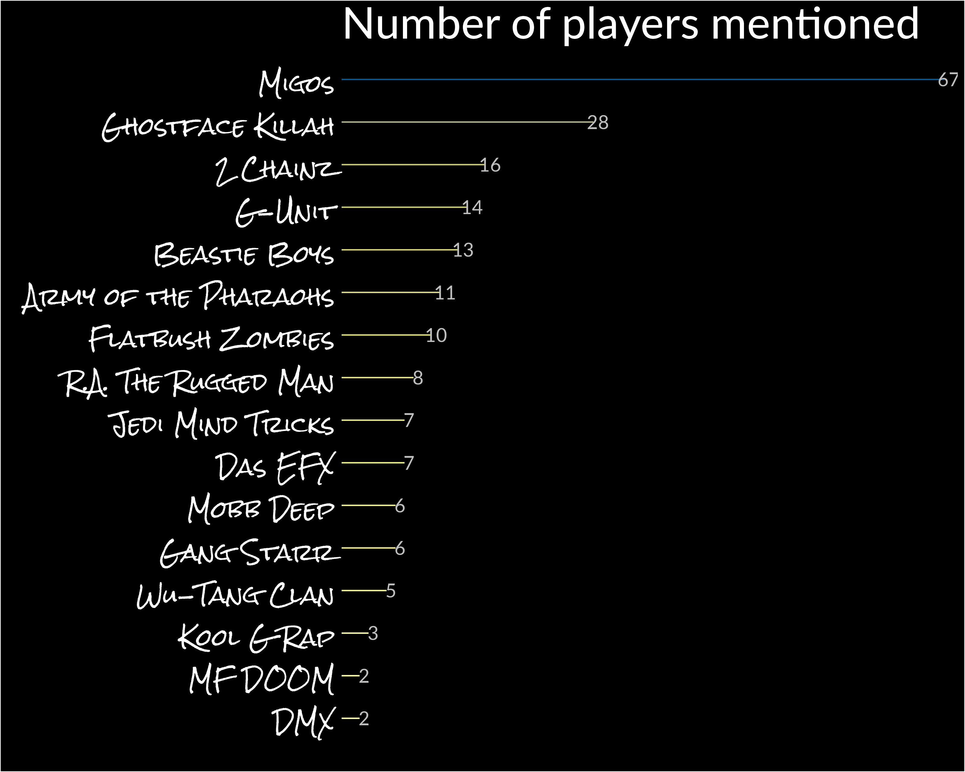
Lastly, for those of us interested in the lines that actually contain player names, we can produce a tibble of artists, song names, and lines by cleaning up the special characters in the line variable and keeping only the rows which contain a name.
# clean weird characters, filter lines to keep mentions only
linesplyrs <-
lyrsplyrs %>% mutate(linecln=str_remove_all(line,"[^\\w\\s]")) %>%
  filter(stringi::stri_detect_regex(linecln,namePlayerBREF)) %>%
  distinct(song_id,.keep_all = TRUE)
A random sample of the lines with player names:
> linesplyrs %>% select(song_name,artist_name,linecln) %>%
+   slice_sample(n=6) %>% as_tibble()
# A tibble: 6 × 3
  song_name                            artist_name      linecln
  <chr>                                <chr>            <chr>
1 Put ’Em In The Grave (Funeral Remix) Jedi Mind Tricks I take my Glock and I point god point guard like Brevin Knight
2 The Black Diamonds                   Ghostface Killah Like Mike Harris
3 Can’t Go Out Sad                     Migos            Quavo Paul Pierce em whip a ball Wilson
4 Drip (Remix)                         Migos            No Vince Carter fifteen with the carbon
5 Look at My Dab                       Migos            Michael Jordan Im perfecting my craft
6 Represent the Real                   Das EFX          This for my block handlin rock like Kenny Anderson
Nice!
This simplistic approach was for a limited number of artists, and by matching full names as they appear in the player dictionary (without considering nicknames, partial matches, or abbreviations) I’m missing out on many more mentions. Still, this code should document a few things I needed to learn such as ranking groups, slicing every other row, text sizing, and colorful annotations.
As usual, feel free to contact me with any questions or comments.