

Bold indicates negative
Late last year I added functionality to unheadr for importing and working with formatted spreadsheet data (see this post).
Recently, I saw this tweet by Mara Averick mentioning a spreadsheet in which bold text = negative values. The unheadr::annotate_mf function can translate cell formatting into text annotations within a data frame or tibble, but only for one target variable at a time.
Based on true events of this afternoon...
— Mara Averick (@dataandme) April 29, 2020
I know, I know there's @nacnudus' {unpivotr}, but seriously?! 🤬
I know, @ChelseaParlett, it's not exactly #statsTikTok, but the feels are real! pic.twitter.com/QbngGYLoPd
After also seeing some COVID-related spreadsheets where bold = negative, it seemed like a good idea to generalize the approach and have a single function that annotates meaningful formatting for all the cells in all the columns of a spreadsheet.

Introducing annotate_mf_all()
annotate_mf_all is now part of unheadr (dev version). Install from GitHub if you haven’t already.
Let’s try it out with the example data bundled with the package. It is an .xlsx file that looks like this.
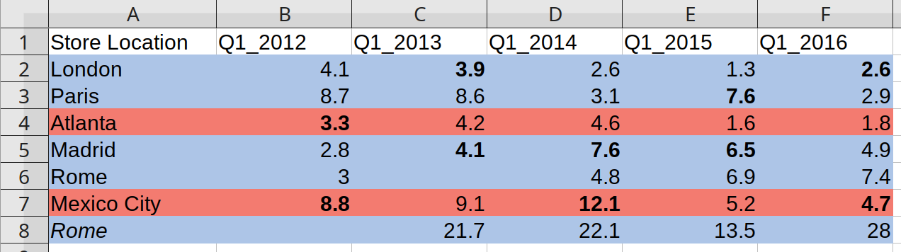
boutiques.xlsx is toy dataset with Q1 profits for different store locations. Additional information is encoded as meaningful formatting. Bold indicates losses (negative values), colors indicate continent, and italic indicates a second location in the same city.
If we know what the different formatting options represent, and have them embedded as text within each cell (value) in an R object, we can parse the formatting and do some cleanup following a relatively simple workflow. A walkthrough:
Load the relevant packages and data
# remotes::install_github("luisdva/unheadr")
library(unheadr) # [github::luisdva/unheadr] v0.2.2.9000
library(dplyr) # [github::tidyverse/dplyr] v0.8.99.9003
library(stringr) # CRAN v1.4.0

# load bundled spreadsheet
sales_spreadsheet<- system.file("extdata/boutiques.xlsx", package = "unheadr")
The new annotate_mf_all function has one argument, a path to a single-sheet spreadsheet (for now), and its output is a tibble with the cell contents and their respective annotations.
# annotate all cells
sales <- annotate_mf_all(sales_spreadsheet)
sales
Let’s see:
> sales
# A tibble: 7 x 6
  `Store Location`    Q1_2012     Q1_2013     Q1_2014     Q1_2015     Q1_2016
  <chr>               <chr>       <chr>       <chr>       <chr>       <chr>
1 (highlighted-FFADC… (highlight… (bolded, h… (highlight… (highlight… (bolded, h…
2 (highlighted-FFADC… (highlight… (highlight… (highlight… (bolded, h… (highlight…
3 (highlighted-FFF37… (bolded, h… (highlight… (highlight… (highlight… (highlight…
4 (highlighted-FFADC… (highlight… (bolded, h… (bolded, h… (bolded, h… (highlight…
5 (highlighted-FFADC… (highlight… (highlight… (highlight… (highlight… (highlight…
6 (highlighted-FFF37… (bolded, h… (highlight… (bolded, h… (highlight… (bolded, h…
7 (italic, highlight… (highlight… (highlight… (highlight… (highlight… (highlight…
All these annotations can be matched with regular expressions to wrangle the data into shape.
# cell colors to indicator variable
sales <-
  sales %>% mutate(region = if_else(str_detect(`Store Location`, "FFADC5E7"), "Europe", "Americas"))
# remove color codes
sales <-
  sales %>% mutate(across(everything(), str_remove, c("highlighted-FFADC5E7|highlighted-FFF37B70")))
Looking better:
> sales
# A tibble: 7 x 7
  `Store Location` Q1_2012       Q1_2013       Q1_2014        Q1_2015       Q1_2016      region
  <chr>            <chr>         <chr>         <chr>          <chr>         <chr>        <chr>
1 () London        () 4.1        (bolded, ) 3… () 2.6         () 1.3        (bolded, ) … Europe
2 () Paris         () 8.7        () 8.6        () 3.1         (bolded, ) 7… () 2.9       Europe
3 () Atlanta       (bolded, ) 3… () 4.2        () 4.6         () 1.6        () 1.8       Americ…
4 () Madrid        () 2.8        (bolded, ) 4… (bolded, ) 7.6 (bolded, ) 6… () 4.9       Europe
5 () Rome          () 3          () NA         () 4.8         () 6.9        () 7.4       Europe
6 () Mexico City   (bolded, ) 8… () 9.1        (bolded, ) 12… () 5.2        (bolded, ) … Americ…
7 (italic, ) Rome  () NA         () 21.7       () 22.1        () 13.5       () 28        Europe
Now we can use a conditional mutate to sort out instances of bold=negative (note the new syntax), and after some minor cleanup we have a usable, rectangular dataset.
# bold = negative
sales <-
  sales %>% mutate(across(Q1_2012:Q1_2016, str_replace, "^\\(bold.+\\)\\s", "-"))
# cleanup brackets
sales <-
  sales %>% mutate(across(everything(), str_remove, "^\\(.*\\)\\s"))
# re-read variable types
sales <- type.convert(sales)
sales
Much better, and now we can actually work with these data (e.g. get totals, means, top and bottom values, etc.)
> sales
# A tibble: 7 x 7
  `Store Location` Q1_2012 Q1_2013 Q1_2014 Q1_2015 Q1_2016 region
  <fct>              <dbl>   <dbl>   <dbl>   <dbl>   <dbl> <fct>
1 London               4.1    -3.9     2.6     1.3    -2.6 Europe
2 Paris                8.7     8.6     3.1    -7.6     2.9 Europe
3 Atlanta             -3.3     4.2     4.6     1.6     1.8 Americas
4 Madrid               2.8    -4.1    -7.6    -6.5     4.9 Europe
5 Rome                 3      NA       4.8     6.9     7.4 Europe
6 Mexico City         -8.8     9.1   -12.1     5.2    -4.7 Americas
7 Rome                NA      21.7    22.1    13.5    28   Europe
Hopefully I can submit this patch to CRAN soon, but please try this out with your own spreadsheets and feel free to send me any feedback.