High-latitude maps

Versión en español

This is a brief guide for making maps in R using ggplot2 and sf, tailored specifically for showing high latitude regions effectively. The example data for this are points that show the distribution of two species of seal near the Antarctic peninsula.

We’ll download observation records for Weddell and Southern elephant seals from gbif through rgbif and coastline data from Natural Earth with rnaturalearth, and plot them with a nice equal-area Azimuthal projection. Working with a suitable projection can really show the location of this study area in context. Projection parameters come from the Projection Wizard web app, based on John P. Snyder’s selection guideline and implemented by the Cartography and Geovisualization Group at Oregon State University.

Let’s go.

Load packages and download the seal observation data for Southern elephant seals and Weddell seals (querying only points for Chile, Argentina, and Antarctica, using their ISO codes and a semicolon to concatenate the query).

# load packages 
library(sf) # CRAN v0.9-1
library(rnaturalearth) # CRAN v0.1.0
library(ggplot2) # CRAN v3.3.0
library(dplyr) # [github::tidyverse/dplyr] v0.8.99.9002
library(rgbif) # CRAN v2.2.0
library(ggimage) # CRAN v0.2.8

# get occurrence data
mlseals <- occ_data(scientificName = "Mirounga leonina",country = "AR;CL;AQ")
wseals <- occ_data(scientificName = "Leptonychotes weddellii",country = "AR;CL;AQ")
mlsealsdat <- mlseals$data
wsealsdat <-wseals$data

Now we coerce the data into simple feature objects, simply by specifying which variables hold the coordinates, and what projection they’re in. Here I decided to subset the data by longitude and latitude, before projecting the combined sf object and creating a buffered bounding box that is used for plotting later on.

# coerce to simple features objects and subset by lat/long
mlsealssf <- 
  mlsealsdat %>% select(scientificName,decimalLongitude,decimalLatitude) %>% 
  distinct() %>% dplyr::filter(decimalLatitude < -40) %>% 
  dplyr::filter(decimalLongitude> -150 & decimalLongitude < -30 )
wsealssf <- 
  wsealsdat %>% select(scientificName,decimalLongitude,decimalLatitude) %>% 
  distinct() %>% dplyr::filter(decimalLatitude < -40) %>% 
  dplyr::filter(decimalLongitude> -150 & decimalLongitude < -30 )

# bind into a single object
sealsdf <- bind_rows(mlsealssf,wsealssf) 

# spatial transformation
seals_spat <- st_as_sf(sealsdf,coords = c("decimalLongitude","decimalLatitude"),crs=4326)               
# proj from Projection Wizard website
sealsproj <- st_transform(seals_spat,"+proj=aea +lat_1=-67.64292238209752 +lat_2=-43.70345673689002 +lon_0=-60.46875")
# arbitrary buffer and bounding box
boundss <- st_bbox(st_buffer(sealsproj,500000))
xydatbuffer <- st_as_sf(st_as_sfc(boundss))

Next, we load country and state polygon outlines from Natural Earth (a public domain map dataset) and project them.

# load country and state outlines and transform 
divpol <- ne_countries(scale = "large",country = c("Chile","Argentina","Antarctica"),returnclass = "sf") %>% 
  st_transform("+proj=aea +lat_1=-67.64292238209752 +lat_2=-43.70345673689002 +lon_0=-60.46875")
regs <- ne_states(country = "Chile",returnclass = "sf") %>% 
  st_transform("+proj=aea +lat_1=-67.64292238209752 +lat_2=-43.70345673689002 +lon_0=-60.46875")
regsAr <- ne_states(country = "Argentina",returnclass = "sf") %>% 
  st_transform("+proj=aea +lat_1=-67.64292238209752 +lat_2=-43.70345673689002 +lon_0=-60.46875")

We are ready to plot all these data as layers in a ggplot call, but to illustrate the use of ggimage and to add some flair to the final map, we can make a table with locations and urls for images that can be drawn over the plot. In this case, little pictures of the two seals drawn by geneticist Julia Saravia and hosted online.

# plotting
# tibble with location and source url for seal drawings
sealimgs <- tibble(x=c(-2023533 ,1725000),y=c(-8200000,-8200000),imgurl=c("https://raw.githubusercontent.com/luisDVA/luisdva.github.io/master/assets/images/pup/mirounga.png",
                                  "https://raw.githubusercontent.com/luisDVA/luisdva.github.io/master/assets/images/pup/wedd.png"))

Ready for plotting. sf does most of the work with the spatial objects. I made a few arbitrary choices for the colors and the plotting extent, mostly for aesthetics.

ggplot()+  
  geom_sf(data=divpol,size=0.2,color="black",fill="#e7d8c9")+
  geom_sf(data=regs,size=0.3,color="black",fill="transparent",lty=2)+
  geom_sf(data=regsAr,size=0.3,color="black",fill="transparent",lty=2)+
  geom_sf(data=sealsproj,pch=21,color="black",aes(fill=scientificName),size=3,stroke=1)+
  geom_image(data=sealimgs[1,],aes(x=x,y=y,image=imgurl),size=0.12)+
  geom_image(data=sealimgs[2,],aes(x=x,y=y,image=imgurl),size=0.14)+
    coord_sf(
    xlim = c(boundss["xmin"]-900000, boundss["xmax"]+900000),
    ylim = c(boundss["ymin"]-800000, boundss["ymax"]))+
  scale_x_continuous(expand = c(0,0))+
  scale_y_continuous(expand = c(0,0))+
  scale_fill_manual(values = c("blue","orange"),name="",labels=c("Southern elephant seal","Weddell seal"))+
  labs(x="",y="")+
  theme(panel.background = element_rect(fill="#c6def1"),
        text = element_text(family = "Loma",size = 18),
        legend.position = "bottom",legend.text = element_text(size = 24))

The plot:

photobomb!

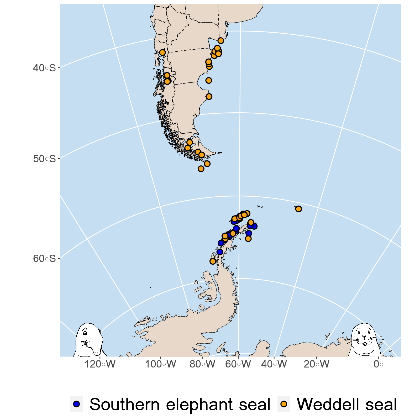
Looks pretty good!
-feedback welcome-