Making sense of trees

In the words of Nick Matzke:

R’s tree structure is pretty non-intuitive, compared to the “a tree is a collection of node objects” structure that is taught in most phylogenetics courses and used in e.g. C++ software. It’s done this way because R likes lists, and doesn’t like objects.

The structure of phylogenetic trees in R (namely APE’s phylo objects) can be confusing because much of the information needed to describe how different nodes and branches make up a tree is implicit.

I learned this the hard way during the early days of my PhD research. My thesis work revolved around phylogenetic lineage ages, so one of my very first tasks after finding a suitable tree was to get a table with species and their ‘edge lengths’ as a way to (more or less) represent their evolutionary ages. At this time I was very new to R and I lost months trying to figure this out on my own. After going over the APE book I slowly realized that lineage age information is contained within the phylo objects and that it can be extracted, but only if you ask nicely.

Phylo objects have a vector of edge lengths for every node, but I was unable to figure out how to get a list of tips and internal nodes that would match up with the vector of edge lengths. After much struggle, I figured out that the branching.times() function computes the distance from each node to the tips, producing a named vector that corresponds to the nodes in the tree. I also learned that the mrca() function produces a matrix of node numbers corresponding to the most recent common ancestors between pairs of tips or nodes. The next challenge would be to put the two together.

I’m writing this brief post because I found an R script from early 2012 in a random USB stick, in which coding superstar Jeff Hanson walked me through indexing, building loops, and functions in order to extract the species lineage ages for any phylogeny object.

The function below has a couple of loops that iterate through the mrca matrix and the branching times vector to produce a data frame of edge lengths for all the tree tips. The for loops make for slow processing if we have large trees but I was patient and that exact function created the main dataset that I analysed for a large part of my thesis. If you’re interested have a look at Jeff’s crisp programming to see how clever he was when coming up with the loops.

# extracting edge lengths from a phylo object
# define function
# note that the function requires ape to be installed

phylLages <- function(inputTree){
require(ape)
# numeric vector with the branching times for each tip
apedates<-branching.times(inputTree)
# matrix of tips and most recent common ancestors
mrca.matrix<-mrca(inputTree)

### preliminary procesing
Species = c()
Node_date = c()

### main processing
col_counter = 0

for (i in colnames(mrca.matrix)) {
  
  # keep track of which column we're in
  col_counter = col_counter + 1
  
  # print messege 
  cat(paste("Starting species ", as.character(col_counter), " out of ", as.character(length(colnames(mrca.matrix))), "\n", sep=""))

  
  # add species name to export vector
  Species = append(Species, i)
  
  # extract a vector of node numbers for the species we're up to
  currNodeVec = mrca.matrix[,col_counter]
  # working out what the node dates are for each node for the species we're working with
  currNodeDates = c()
  row_counter = 0
  for (currNodeNum in currNodeVec) {
    row_counter = row_counter + 1
    if (row_counter != col_counter) {
      currNodeDates = append(currNodeDates, apedates[as.character(currNodeNum)])
    }
  }
  # find out what the minimum number is
  minDate = min(currNodeDates)
  Node_date = append(Node_date, minDate)
  
        }
  exportFrame = data.frame(Species,Node_date)
  cat("DONE!\n")
  return(exportFrame)
}

A few years later I learned that the BioGeoBEARS R package includes the prt() function, which Nick Matzke wrote specifically to print the content of a tree into a tabular format, making all the implicit information explicit. This function is faster and provides much more information, and I was very relieved to see that the edge lengths it provides are the same Jeff and I obtained with the custom function.

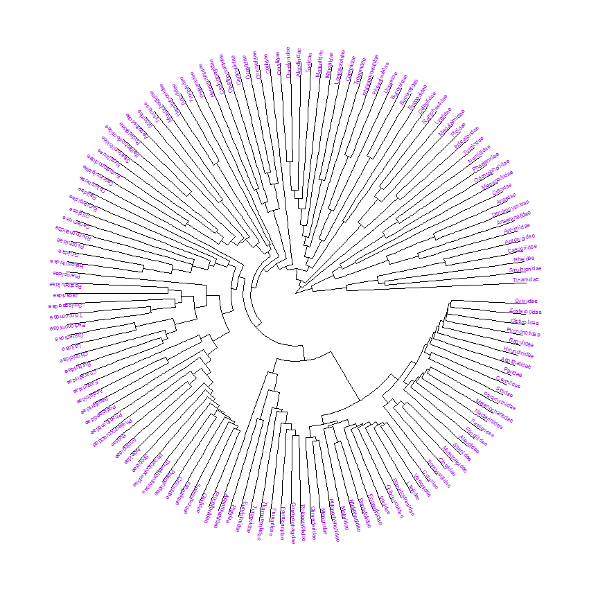
Lets have a look. Both functions keep the tip order so comparing the results is easy. This examples uses the built in tree of bird families (Sibley and Ahlquist 1990) from the ape package.

plotted with ggtree

# comparing the edge lengths with BioGeoBEARS::prt

# load libraries
library(ape)
library(dplyr)
library(stringr)
library(BioGeoBEARS)

# phylogeny of bird families (comes with ape)
data("bird.families")

# get a data frame of edge lengths using the Jeff Hanson & Luis Verde function
jhEdges <- phylLages(bird.families)

# get a data frame of edge lengths using prt
birdPrintout <- prt(bird.families)
## extract the data for the tips only
# note: the tips in this particular tree are families not species 
birdPrintout_Tips <- birdPrintout %>% filter(str_detect(label,"Node")==FALSE) %>% 
                        select(Species=label,Node_date=edge.length)
# quick comparison
head(jhEdges) == head(birdPrintout_Tips)
 

Now we can do side-by-side glimpse of the two data frames, and time how long the two functions take to process the data.

> bind_cols(jhEdges,birdPrintout_Tips) %>% head
        Species Node_date       Species Node_date
1 Struthionidae      17.1 Struthionidae      17.1
2       Rheidae      17.1       Rheidae      17.1
3   Casuariidae       9.5   Casuariidae       9.5
4   Apterygidae       9.5   Apterygidae       9.5
5     Tinamidae      21.8     Tinamidae      21.8
6      Cracidae      19.8      Cracidae      19.8

system.time(phylLages(bird.families))
system.time(prt(bird.families))

prt is about 4.5x faster than the loops, and this becomes relevant as the number of tips increases or in the case of multiphylo objects with varying edge lengths so I recommend using it for any work on edge lengths.