
Versión en español aquí
Nowadays, it is not only possible but also straightforward to make cool and informative 3d maps in R. Thanks to rayshader and rayrender by Tyler Morgan-Wall and elevatr by Jeff Hollister, we can combine a georeferenced image and a Digital Elevation Model (DEM) to really bring an existing map to life.
Twitter user @flotsam has many great examples, such as this recent one:
A 1972 NRCan (formerly the Department of Energy, Mines, and Resources) map of Montréal, Canada. Spent more time trying to decipher cryptic filenames to find what I want than actually rayshading it. :P#rayshader adventures, an #rstats tale pic.twitter.com/O756ddhs9G
— flotsam (@researchremora) August 2, 2021
The overall process for rayshading a georeferenced image is summarized step-by-step in this gist by Tyler Morgan-Wall.
There are many georeferenced maps online, and we can use GIS software to match up any digital map with its corresponding spatial context by creating ground control points. However, I like making my own thematic maps in ggplot2 and wanted to plot one in 3d with rayshader.
To make maps in ggplot2 using popular spatial packages (sf, stars, etc.), we are already working with spatial data, so there should be no need to assign real-world coordinates to each pixel of the raster in the final map manually. I also kept losing my patience trying to create control points for a polynomial warp using a trackpad or the weird orange nub on my computer with my shaky hand.
This StackOverflow thread explains how to pull the information that describes the maximum and minimum xy values for the panel in a ggplot object and then assign them to the raster image we exported this object as.
If we want to avoid manual georeferencing and use this approach, the key point here (which is kind of a hack) is to make sure that the ggplot object has no margins so that the xy values that describe the panel extent match up with the overall extent of the image we export and then use for rayshader. For this, we can use a custom theme (theme_nothing) that comes with the cowplot package by Claus Wilke, and the rationale is explained here. Basically, this theme is equivalent to setting various plot elements to blank with no expansion of the scales.
Let me demonstrate. This example uses spatial data from the CONABIO Geoinformation Portal and the CONANP spatial Information download area. I downloaded shapefiles for Protected Areas (Áreas Naturales Protegidas ) and Landcover types (Uso del suelo y vegetación, escala 1:250000, serie VI (continuo nacional)) and then focused on the Iztaccíhuatl-Popocatépetl protected area.
These steps are for reading the shp data, subsetting the features for the area of interest, lumping together some of the land cover categories (somewhat arbitrarily) with case_when and making a simple map of the volcanoes with pretty colors that I chose for each land cover type. Note how theme_nothing() removes all the margins and axis ticks/labels, and then I added extra arguments to coord_sf() to make sure everything stays within the plot panel.
# load packages
library(sf)        # CRAN v0.9-8
library(dplyr)     # CRAN v1.0.7
library(stringr)   # CRAN v1.4.0
library(ggplot2)   # CRAN v3.3.3
library(raster)    # CRAN v3.4-13
library(stars)     # [github::r-spatial/stars] v0.5-3
library(elevatr)   # CRAN v0.4.1
library(rayshader) # [github::tylermorganwall/rayshader] v0.26.1
library(smoothr)   # CRAN v0.2.2

# import ANP data
anps <- st_read("YOUR-PATH-HERE/182ANP_Geo_ITRF08_Agosto_2020.shp") %>%
  dplyr::select(NOMBRE)

# import vegetation
veg <- st_read("YOUR-PATH-HERE/usv250s6gw.shp") %>%
  st_transform(st_crs(anps))

# feature of interest
izta <- anps %>% filter(str_detect(NOMBRE, "Izt"))

# map limits
Iztbbox <- st_buffer(izta, dist = 0.1) %>%
  st_bbox() %>%
  st_as_sfc()

# summarize vegetation
veggr <- veg %>%
  group_by(CVE_UNION) %>%
  summarize(.groups = "keep")

# crop vegetation to limits
Iztveg <- st_crop(veggr, Iztbbox)

# re-classify vegetation types
Iztvegrc <- Iztveg %>% mutate(vegclass = case_when(
  str_detect(CVE_UNION, "^B") ~ "Bosque",
  str_detect(CVE_UNION, "^VS") ~ "Vegetación secundaria",
  str_detect(CVE_UNION, "^T") ~ "Agricultura (temporal)",
  str_detect(CVE_UNION, "^R") ~ "Agricultura (Riego)",
  str_detect(CVE_UNION, "DV") ~ "Sin vegetación",
  str_detect(CVE_UNION, "^P") ~ "Pastizal",
  str_detect(CVE_UNION, "VW") ~ "Pradera de alta montaña",
  TRUE ~ CVE_UNION
))

# smooth vegetation features
Iztvegrc <- smooth(Iztvegrc)

# set up graphics device
ragg::agg_tiff(
  filename = "izt.tiff",
  res = 400, width = 3.88, height = 5.92, units = "in"
)
# plot
iztgg <-
  ggplot() +
  geom_sf(data = Iztvegrc, aes(fill = vegclass), size = 0) +
  scale_fill_manual(values = c(
    "#b5c99a", "#97a97c", "#8d99ae", "#26432F",
    "#e8e8e4", "#cdeac0", "#B1D5BB",
    "#cde5d7", "#adb6c4", "#9cc5a1",
    "#ffc49b", "#eaeaea", "#f3e7e4"
  ), guide = FALSE) +
  ggfx::with_outer_glow(geom_sf(data = izta, fill = "transparent", color = "white", size = 0.1),
    expand = 3, colour = "white"
  ) +
  coord_sf(expand = FALSE, clip = "on") +
  cowplot::theme_nothing() +
  theme(
    panel.grid.major = element_line(color = "#14213d", size = 0.1, linetype = "dashed"),
    panel.ontop = TRUE
  )

iztgg

dev.off()
It took some trial and error to export the tiff (using a ragg device) and have no blank space around the edges, but once the output looks good we can read this new image with the raster package.
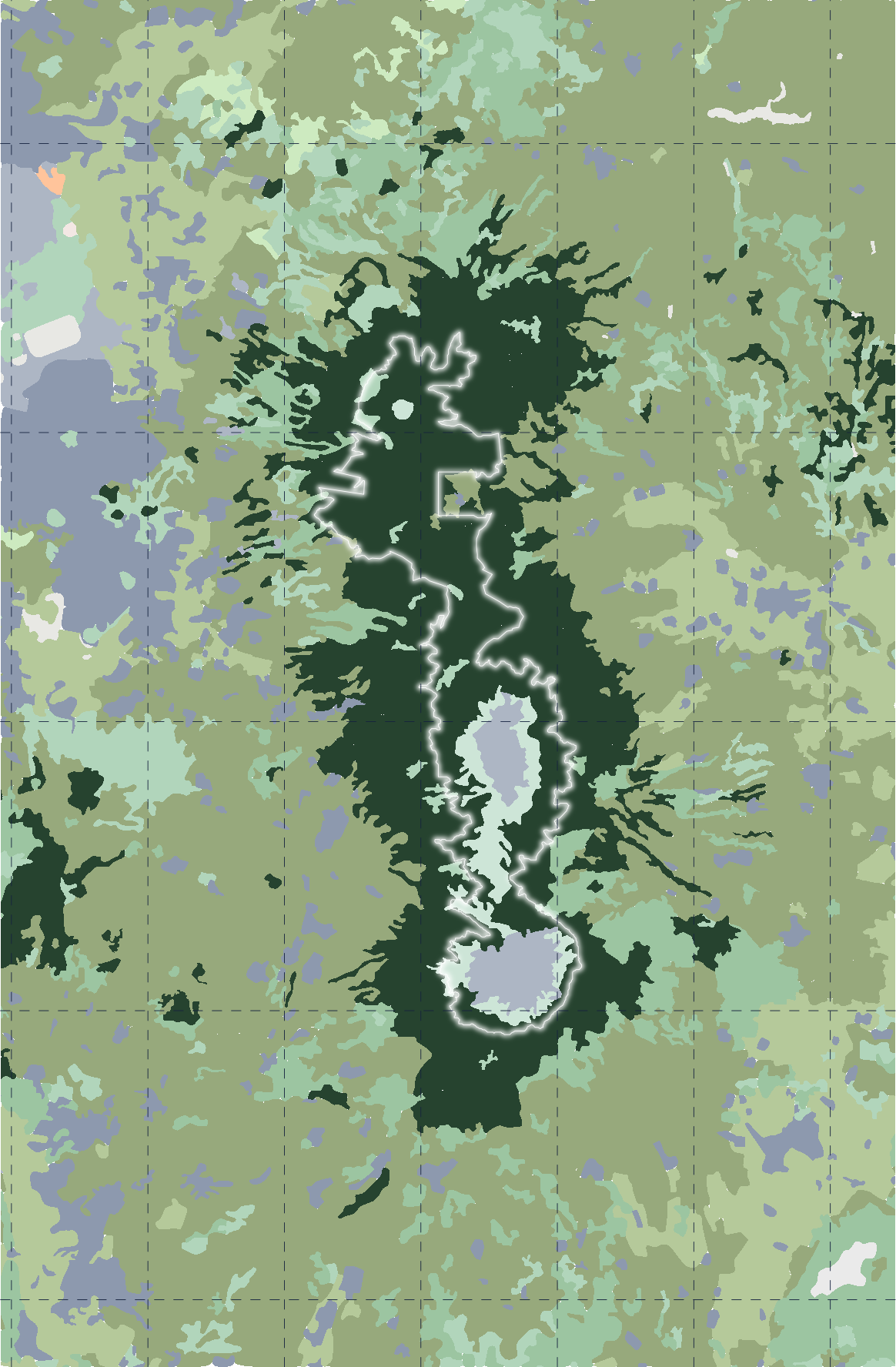
Let’s import the tiff and have a look.
# Create a StackedRaster object from the saved plot
stackedRaster <- raster::stack("izt.tiff")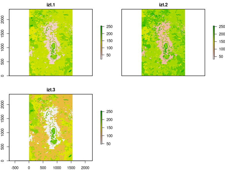
The geospatial data we need is in the ggplot object, and we can pull it out with ggplot_build and some indexing. This gives us a list with ranges for x and y, which go into the extent function to finally georeference the map (we also need to define the projection). Next, we export the georeferenced raster. INT1U means the values are bound between 0 and 255, and PHOTOMETRIC=RGB is the color interpretation tag.
# Get the GeoSpatial Components
lat_long <- ggplot_build(iztgg)$layout$panel_params[[1]][c("x_range", "y_range")]

# Supply GeoSpatial  data to the StackedRaster
raster::extent(stackedRaster) <- c(lat_long$x_range, lat_long$y_range)
raster::projection(stackedRaster) <- raster::crs(st_crs(Iztvegrc)$proj4string)

# write to disk
writeRaster(stackedRaster, "iztGeoTiff.tif", options = "PHOTOMETRIC=RGB", datatype = "INT1U", overwrite = TRUE)
Let’s re-import the geoTiff
# reread
grRast <- raster::brick("iztGeoTiff.tif")
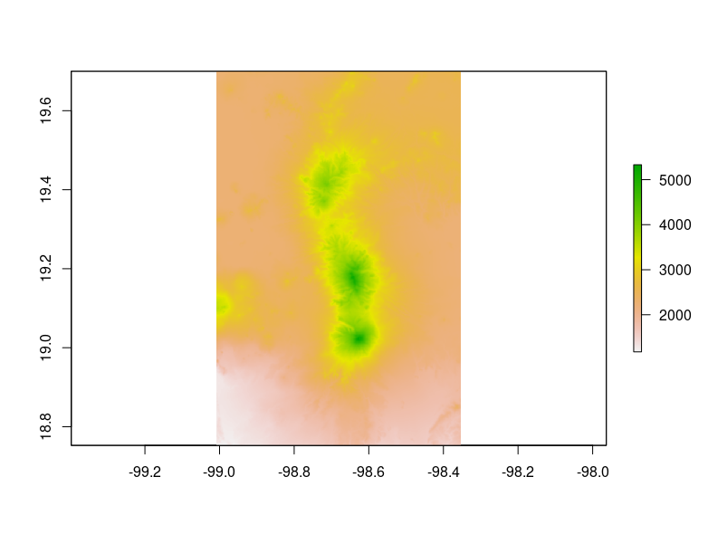
grRastst <- raster::stack(grRast)After this, the process follows most guides on rayshading images. First, we transform the raster to an array and use it to get elevation data using elevatr. We will then crop, resize, and transpose the DEM data (because rasters and arrays are oriented differently in R).
# to array for draping
test_c_arr <- as.array(grRastst)

# get elevation data
Rch_dem <- elevatr::get_elev_raster(grRastst, z = 9)
Rch_dem <- raster::crop(Rch_dem, grRastst)
plot(Rch_dem)

# Reduce the size of the elevation data, for speed
areademMatrix <- rayshader::resize_matrix(rayshader::raster_to_matrix(Rch_dem), scale = 0.7)

# transpose
demFinal <- (areademMatrix)
A quick glimpse of the elevation data
Now we can compute the shadows and drape the array on the elevation data.
# Compute shadows
ambient_layer <- ambient_shade(demFinal, zscale = 10, multicore = TRUE, maxsearch = 200)
ray_layer <- ray_shade(demFinal, zscale = 20, multicore = TRUE)
# Plot in 3D
(test_c_arr / 255) %>%
add_shadow(ray_layer, 0.3) %>%
add_shadow(ambient_layer, 0) %>%
plot_3d(demFinal,
zscale = 150, theta = -50, phi = 28, zoom = 0.3,
windowsize = c(1200, 800), solid = FALSE,
background = "#3d314a"
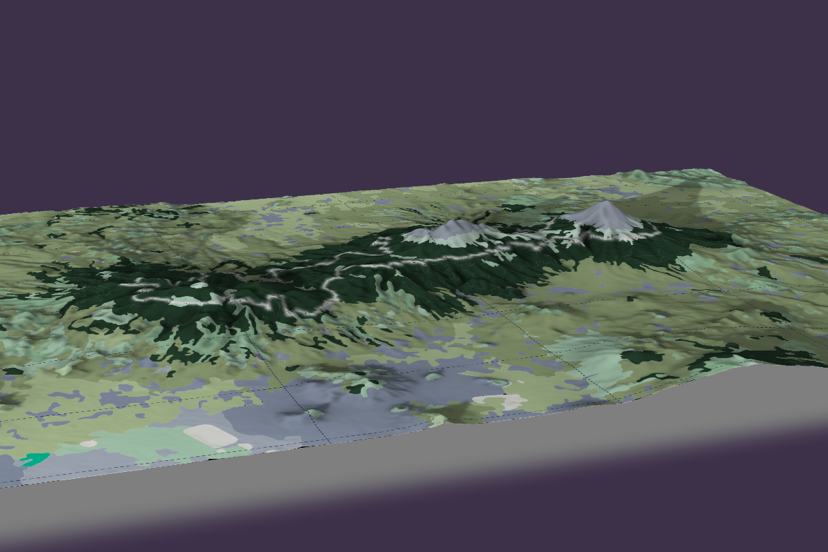
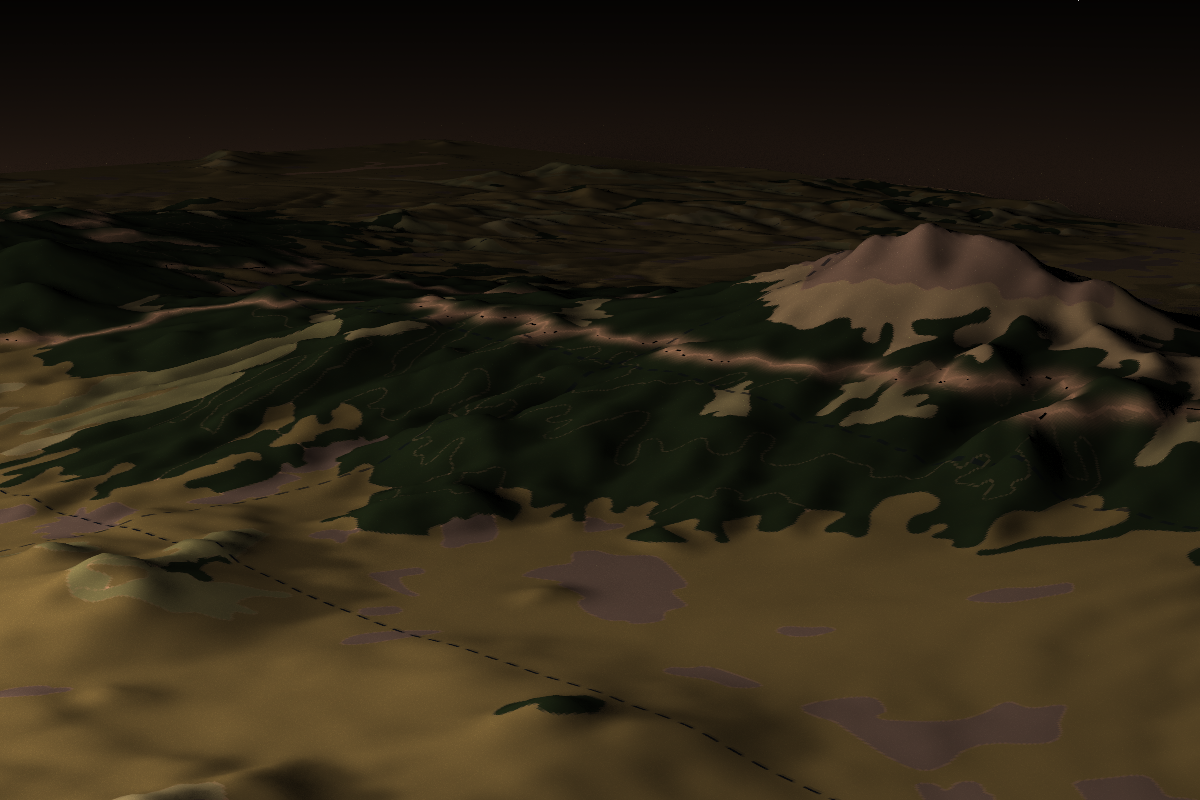
)Here’s a snapshot of the rgl window produced by plot3d, after fiddling with the camera values. If you are reading this in Mexico City, the area should look familiar.
An overhead view produced by plot_map() looks pretty good too.
# Plot in 2D
(test_c_arr / 255) %>%
  add_shadow(ray_layer) %>%
  add_shadow(ambient_layer, 0) %>%
  plot_map()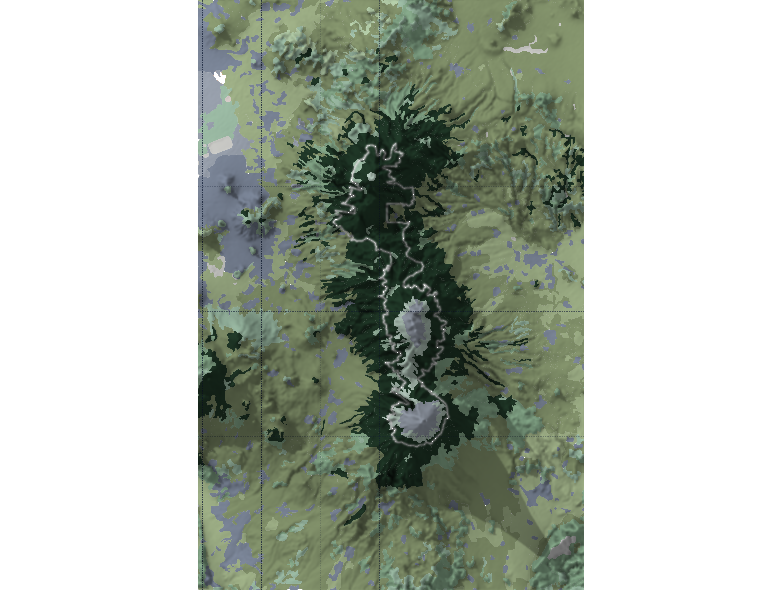
Finally, we can add elements with rayrender and render the fancier maps with render_highquality(). I like this approach to add more atmosphere by using light = FALSE and instead lighting the scene with a sphere of light placed at a custom location.
Turn off the lights and add your own🤓: #rstats #rayshader #rayrender
— Tyler Morgan-Wall (@tylermorganwall) October 27, 2019
render_highquality(light = FALSE, scene_elements = sphere(y = 100, radius = 10, material = diffuse(lightintensity = 250, implicit_sample = TRUE))) pic.twitter.com/g1QDEphZGh
# render with 'golden' light
render_highquality(
light = FALSE,
scene_elements = rayrender::sphere(
z = 450, y = 100, x = 200, radius = 36,
material = rayrender::light(
intensity = 150,
spotlight_width = 20,
color = "#ff773d"
)
)
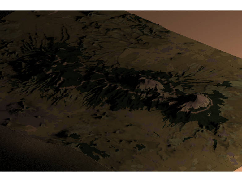
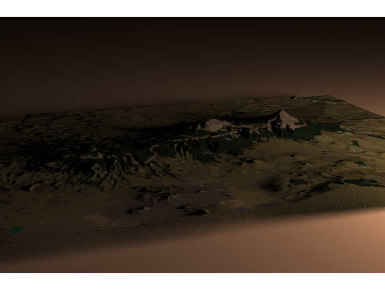
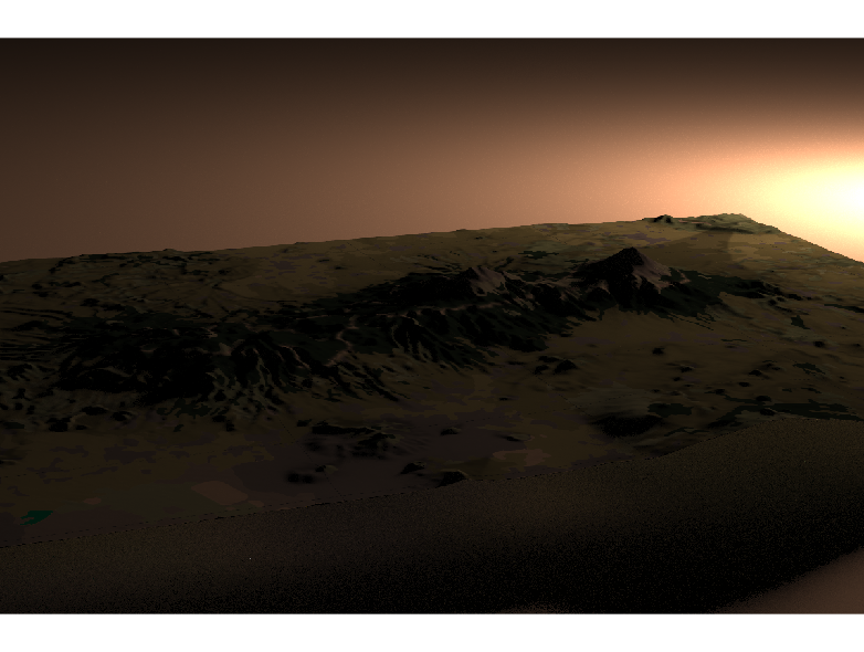
)Here are some renders with different camera locations and light placements.
The results came out quite nice, and with this setup we could even make animations or add additional elements. This approach can also work with base R plots, as long as the plot panel goes all the way to the edges of the output raster image. I hope someone finds this helpful or entertaining. If you have any questions or feedback please let me know.